📦 Part 4 of Build Your Own Quant Research System — follow the series and you’ll build a complete, modular research toolkit from scratch, one tutorial at a time.
✅ Tested: vectorbt 1.1.1 · Python 3.12 · Last verified: 2026-10-08 · Update policy
📊 Market snapshot (as of 2026-10-08): SPY $777.22 · QQQ $757.73 · BTC $83,172 · ETH $2,580 — for context on when this was written.
In Part 1 we backtested a moving-average crossover and got Sharpe 1.03. In Part 2 we showed that number drops to 0.36 out-of-sample. Painful, but at least honest.
This tutorial goes one level deeper. Part 2 asked: “does the strategy work on unseen data?” Part 4 asks a nastier question: “you tried 142 parameter combinations and picked the best — how much of that ‘best’ is just luck?”
The answer, it turns out, is “most of it.” And there are two statistical tools that prove it: the Deflated Sharpe Ratio and PBO (Probability of Backtest Overfitting). This tutorial gives you both — the intuition, the code, and the uncomfortable numbers for our own MA grid.
Risk note: Everything here is educational. Backtests are hypothetical — they don’t predict future returns, and statistical significance doesn’t mean a strategy is tradable. Nothing in this article is investment advice.
1. The Multiple Testing Trap
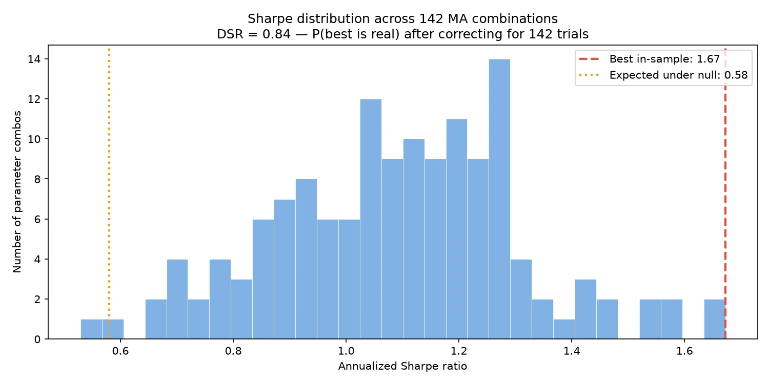
Here’s the setup. You have an idea — say, moving-average crossover. You don’t know the best parameters, so you test a grid: fast MA from 5 to 50, slow MA from 20 to 100, every combination where fast < slow. That’s 142 backtests.
You pick the winner. Sharpe 1.67. You feel great.
Here’s the problem: you didn’t run one backtest. You ran 142, and reported the maximum. That maximum is a biased estimator — it’s the best of 142 draws, and even if every single strategy is pure noise, the best of 142 noise draws looks impressive.
Think of it this way: flip a coin 10 times, 100 different coins. One of them will show 8+ heads just by chance. Would you conclude that coin is “biased toward heads”? Of course not. But that’s exactly what “pick the best Sharpe of 142” does.
The finance literature has a name for this: selection bias under multiple testing. And the standard correction is the Deflated Sharpe Ratio (Bailey & López de Prado, 2014).
The key insight: the more trials you run, the higher the bar for “significant.” A Sharpe of 1.5 might be excellent if it’s your first test. If it’s the best of 500 tests, it’s probably noise. DSR quantifies exactly how much to discount.
2. Deflated Sharpe Ratio
The Deflated Sharpe Ratio answers one question: “What’s the probability that the true Sharpe ratio is positive, after accounting for the fact that I cherry-picked the best of K trials?”
The intuition (no formula dump)
Imagine K researchers each test one random strategy on the same data. Each gets a Sharpe ratio — mostly near zero, some positive, some negative, just noise. Now take the maximum of those K Sharpes. That maximum has an expected value even when there’s zero real edge — call it SR₀ (the “null” Sharpe).
DSR compares your observed Sharpe against SR₀:
– Observed >> SR₀: your Sharpe is surprisingly high even for the best-of-K. Probably real.
– Observed ≈ SR₀: your “great” result is exactly what you’d expect from picking the best noise. Probably luck.
SR₀ grows with K (more trials → higher expected maximum) and with the variance of trial Sharpes (noisier trials → luckier winners).
What DSR gives you
A probability between 0 and 1:
– DSR > 0.95: statistically significant. The Sharpe survives the multiple-testing correction.
– DSR 0.5–0.95: marginal. Might be real, might not. Get more data or fewer trials.
– DSR < 0.5: the backtest is likely luck. The “best” strategy is the luckiest noise.
The code
from overfitting import deflated_sharpe

# Best of 142 trials, Sharpe 1.67, 752 daily bars
dsr = deflated_sharpe(
    observed_sr=1.67,
    trial_srs=all_142_sharpes,  # every trial, not just the best
    n_obs=752,
)
print(f"DSR = {dsr:.3f}")  # 0.840 — marginal, not significant
The critical input is trial_srs — all K Sharpe ratios, not just the winner. DSR needs the full distribution to estimate how lucky the winner got. If you only saved the best result and threw away the other 141, you can’t compute DSR. (Lesson: always save every trial.)
The full implementation is in overfitting.py, following Bailey & López de Prado (2014) exactly — including the skewness/kurtosis correction for non-normal returns.
3. PBO: Probability of Backtest Overfitting
DSR asks “is my best Sharpe real?” PBO asks a different question: “if I pick the best strategy in-sample, how likely is it to disappoint out-of-sample?”
The intuition
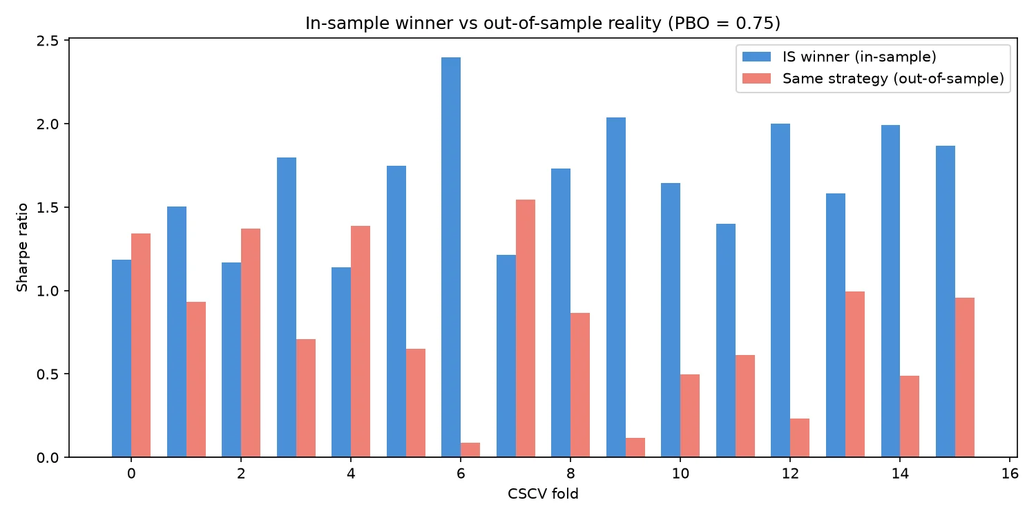
López de Prado’s insight (Advances in Financial Machine Learning, ch. 11): split your history into blocks. For many different in-sample/out-of-sample splits, find the IS winner and check its OOS rank. If the IS winner consistently ranks below median OOS, your selection process is overfitting — you’re picking noise, not signal.
It’s called “Combinatorial Symmetric Cross-Validation” (CSCV) because it uses many complementary IS/OOS partitions. The “probability” in PBO is the fraction of folds where the IS-optimal strategy lands below the OOS median.
- PBO near 0: the IS winner usually holds up OOS. Selection is working.
- PBO near 0.5+: the IS winner is no better than random OOS. You’re overfitting.
Simplified vs the paper
The original PBO fits a logit model on rank pairs and integrates — powerful but complex. Our pbo() uses a simplified version: directly count the fraction of CSCV folds where the IS winner ranks below the OOS median. Same intuition, fewer moving parts. For production decisions, read AFML chapter 11.
from overfitting import pbo

# returns_matrix: (n_strategies, n_periods) — one row per variant
result = pbo(returns_matrix, n_partitions=8)
print(f"PBO = {result['pbo']:.3f}")  # 0.750 — overfit
print(f"Folds: {result['n_folds']}")
4. Reality Check: Our MA Grid
Time for honest numbers. Same SPY data as Part 1 (752 daily bars, October 2023 to October 2026). Grid: 142 MA(fast, slow) combinations.
In-sample (pick the best of 142):
| Metric | Value |
|---|---|
| Best combo | MA(20, 25) |
| Sharpe | 1.67 |
| Trials | 142 |
Looks fantastic. Now the corrections:
Deflated Sharpe Ratio: 0.84. Not significant at the 0.95 level. The 1.67 is marginal — it could be real, but after correcting for 142 trials, we can’t rule out luck. The expected Sharpe of the best-of-142 noise draws (SR₀) was high enough to explain most of the 1.67.
PBO (simplified): 0.75 over 16 folds. The in-sample winner ranked below the OOS median in 75% of folds. That’s a strong overfitting signal — the selection process is picking noise more often than not.
Three takeaways:
-
1.67 → 0.84 is the multiple-testing discount. The raw Sharpe is meaningless without knowing K. Always report DSR (or equivalent) alongside the best Sharpe. If someone shows you a Sharpe without telling you how many trials they ran, assume the worst.
-
PBO 0.75 means the grid search is mostly noise-mining. With 142 combinations on 3 years of data, we’re slicing too thin. Fewer trials, more data, or stronger priors (fewer degrees of freedom) would all help.
-
This doesn’t mean MA crossover is useless. It means this specific selection process (142 combos, pick best Sharpe) doesn’t produce reliable winners. A simpler approach — pick (20, 50) from theory, don’t optimize — avoids the multiple-testing trap entirely. Sometimes the best optimization is no optimization.
Run it yourself: overfitting_demo.py reproduces every number above.
5. Merge Into the Toolkit: overfitting.py
This tutorial isn’t a standalone trick — it’s Part 4 of a system we’re building together. The overfitting statistics now live as the fourth module of goosos/quant-toolkit:
from quant_toolkit.backtest import run_backtest, ma_crossover_signals
from quant_toolkit.validation import run_walk_forward
from quant_toolkit.overfitting import deflated_sharpe, pbo

# The Part 1 number (in-sample, best of K)
print("best Sharpe:", trial_srs.max())

# The Part 4 correction (is it real?)
print("DSR:", deflated_sharpe(trial_srs.max(), trial_srs, n_obs=len(price)))
print("PBO:", pbo(returns_matrix)["pbo"])
Why a toolkit, not just scripts? Each tutorial in this series adds one module. By Part 10 you’ll have backtest, validation, data, overfitting, metrics, costs, and sizing — a research system you understand line by line, because you watched every line get written. That’s the difference between using a library and owning your process.
Next: Part 5: Performance Metrics Deep Dive adds
metrics.py— beyond Sharpe: Sortino, Calmar, and when each one lies.
FAQ
DSR vs regular t-test on the Sharpe — what’s the difference?
A t-test asks “is this Sharpe significantly positive?” assuming it’s the only test you ran. DSR asks the same question given that you picked the best of K. With K=1, DSR reduces to the standard test. With K=142, the bar is much higher.
My DSR is 0.84. Should I trade the strategy?
0.84 means “probably real, but not proven.” It’s not a green light, but it’s not a rejection either. Get more data, reduce trials, or find confirming evidence (walk-forward, different market). Don’t trade on 0.84 alone.
PBO 0.75 seems very high. Is my code wrong?
Probably not — 0.75 is honest for 142 trials on 3 years of data. PBO is high when (a) many trials, (b) short history, (c) noisy strategies. All three apply here. It’s telling you the truth: this grid search is overfit.
Can DSR/PBO be gamed?
Yes — by not reporting all trials. If you run 500 backtests, keep the 10 best, and compute DSR on K=10, you’ll get an inflated DSR. The correction only works if K is honest. This is why we say: save every trial, always.
Why not just use train/test split instead?
Train/test (Part 2’s walk-forward) and DSR/PBO answer different questions. Walk-forward asks “does it work on unseen data?” DSR asks “is the best-of-K result statistically significant?” Use both — they catch different failure modes.
References
- Bailey, D. H., & López de Prado, M. (2014). The Deflated Sharpe Ratio: Correcting for Selection Bias in Backtests. — the DSR paper; source for the formula implemented here.
- López de Prado, M. Advances in Financial Machine Learning (2018), Chapter 11 (Backtest Overfitting) — PBO and CSCV framework.
- goosos/overfitting-tutorial — full code for this article.
- goosos/quant-toolkit — the growing toolkit;
overfitting.pyis the Part 4 module.
Further Reading
- Part 1: VectorBT Tutorial — the backtest this article stress-tests; adds
backtest.py. - Part 2: Walk-Forward Analysis — in-sample vs out-of-sample; adds
validation.py. - Part 3: Data Cleaning & Alignment — garbage in, garbage out; adds
data.py. - Part 5: Performance Metrics Deep Dive (upcoming) — adds
metrics.py.
Part 4 of Build Your Own Quant Research System · Code: goosos/overfitting-tutorial · Toolkit: goosos/quant-toolkit · Next: Part 5: Performance Metrics
