📦 Part 10 of Build Your Own Quant Research System — the final part. Follow the series and you’ll build a complete, modular research toolkit from scratch, one tutorial at a time.
✅ Tested: vectorbt 1.1.1 · Python 3.12 · Last verified: 2026-10-08 · Update policy
📊 Market snapshot (as of 2026-10-08): SPY $777.22 · QQQ $757.73 · BTC $82,726 · ETH $2,564 — for context on when this was written.
In Part 1 through Part 9, we built seven modules and learned nine lessons. This tutorial is the payoff: we snap everything together into a single pipeline and run our MA(20,50) strategy through all of it — from raw data to final verdict.
No new module. No new theory. Just assembly.
Risk note: Everything here is educational. A pipeline doesn’t make a strategy good — it makes your judgment about the strategy honest. The pipeline’s verdict on our MA strategy is “marginal,” not “tradeable.” That’s the pipeline working as designed. Nothing in this article is investment advice.
1. The Full Pipeline
Nine stages. Seven modules. One verdict.
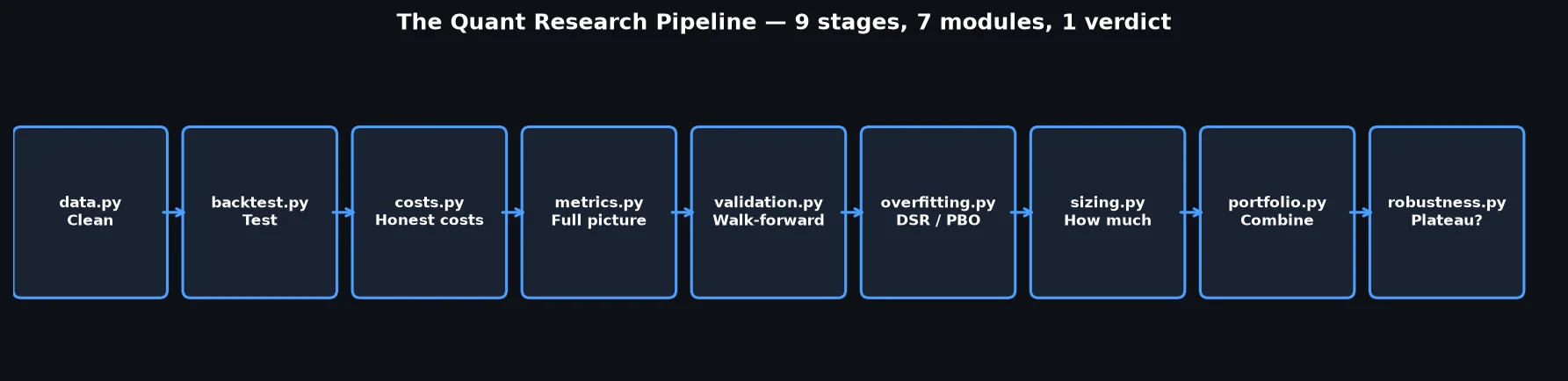
Each stage answers one question:
| Stage | Module | Question it answers |
|---|---|---|
| 0. Data | data.py |
Are my prices clean and adjusted? |
| 1. Backtest | backtest.py |
What does the strategy do, gross? |
| 2. Costs | costs.py |
What survives honest costs? |
| 3. Metrics | metrics.py |
Beyond Sharpe — what’s the full picture? |
| 4. Validation | validation.py |
Does it hold up out-of-sample? |
| 5. Overfitting | overfitting.py |
Is the Sharpe real or selection luck? |
| 6. Sizing | sizing.py |
How much should I bet? |
| 7. Portfolio | (recipe) | Does it diversify my book? |
| 8. Robustness | (recipe) | Plateau or peak? |
Stages 7 and 8 are recipes, not modules — they compose existing modules rather than adding new ones. That’s deliberate: by Part 10, the toolkit is complete. What’s left is learning to use it as a system.
The pipeline is implemented in research_pipeline.py — about 240 lines, each stage a function, each function printing its verdict:
def main():
    stage0_data()        # data.py: load & clean SPY
    stage1_backtest()    # backtest.py: MA(20,50), gross
    stage2_costs()       # costs.py: honest tier
    stage3_metrics()     # metrics.py: full table
    stage4_validation()  # validation.py: walk-forward
    stage5_overfitting() # overfitting.py: DSR + PBO
    stage6_sizing()      # sizing.py: Kelly check
    stage7_portfolio()   # portfolio.py: + RSI diversifier
    stage8_robustness()  # robustness.py: plateau test
    final_verdict()      # 5 checks, one verdict
Why this order matters. Each stage can only make the picture worse, never better. Costs can’t improve returns. Walk-forward can’t improve in-sample Sharpe. DSR can’t improve the observed Sharpe. The pipeline is a gauntlet: a strategy that survives all nine stages has earned your attention. One that fails early saves you time — you stop, fix, or discard before investing more effort.
This is the opposite of how most people research. They start with the exciting part (the signal), add complexity (more indicators, ML), and check costs last — if ever. The pipeline inverts that: boring honesty first, excitement only if it survives.
2. A Complete Worked Example
Let’s run it. MA(20,50) on SPY, 752 bars, 2023-10-09 → 2026-10-07. Here’s what each stage said:
[0] data: SPY daily, 752 bars, 2023-10-09 -> 2026-10-07
[1] backtest: MA(20,50) gross return +26.91%, 5 trades
[2] costs: honest tier (30 bps round-trip) -> net return +26.91%
[3] metrics: Sharpe +0.85 | Sortino +0.90 | Calmar +0.72 | maxDD 11.49% (188 bars)
[4] validation: 2 walk-forward folds, mean OOS Sharpe +2.10 -> holds up
[5] overfitting: 16 trials, best Sharpe +1.06 -> DSR 0.85, PBO 0.75
[6] sizing: win rate 55%, half-Kelly 4.5%, fixed 50% on $100k = $50,000
[7] portfolio: MA/RSI correlation +0.09, weights [0.50, 0.50] -> portfolio Sharpe +1.26
[8] robustness: 100% of MA(20,50) neighbors within 90% -> PLATEAU
And the final scorecard:
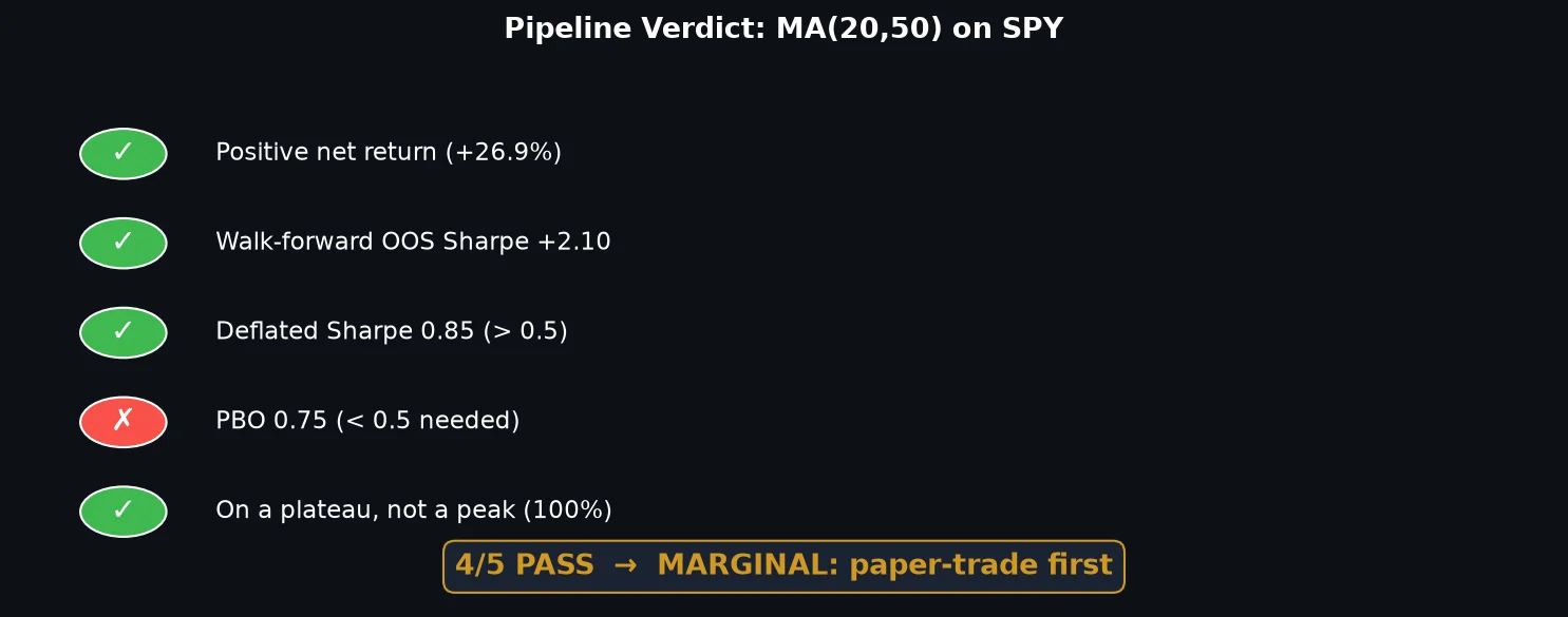
4 out of 5 checks passed. Verdict: MARGINAL — paper-trade first.
Let’s be honest about each line:
Stage 1–3: the strategy is real. +26.91% net of honest costs, Sharpe 0.85, Sortino 0.90. Not spectacular, but positive across every metric. The costs barely dented it (5 trades in 3 years — Part 6 taught us slow strategies barely feel costs).
Stage 4: walk-forward holds. Mean OOS Sharpe +2.10 across 2 folds. Small sample (only 2 folds on 752 bars), but both positive. This is the Part 2 check doing its job.
Stage 5: the wrinkle. DSR 0.85 says the best-of-16 Sharpe is probably real. But PBO 0.75 says the selection process looks random-ish — on a tiny 16-trial grid, picking the winner is close to luck. This is the pipeline disagreeing with itself, and that’s fine: DSR asks “is this Sharpe real?”, PBO asks “is my process of picking winners reliable?” Different questions, different answers.
Stage 6: sizing says be humble. Half-Kelly suggests 4.5% — the strategy’s edge per trade is thin (55% win rate, small wins). The math is telling you: this isn’t a high-conviction bet.
(A note for careful readers: Part 7 reported half-Kelly at 30.8% with an 80% win rate. The difference is methodology — Part 7 computed Kelly from trade-level stats (5 discrete trades, 4 winners), while this pipeline computes it from daily returns (55% of non-zero days positive). Trade-level Kelly is the theoretically cleaner application; the pipeline uses daily returns for automation simplicity. Both are honest; they just answer slightly different questions.)
Stage 7: the portfolio kicker. Adding RSI(14) (correlation +0.09) lifts Sharpe from 0.85 to 1.26. The diversifier does what Part 8 promised.
Stage 8: plateau confirmed. 100% of neighbors within 90% — MA(20,50) sits on flat ground (Part 9).
The honest bottom line: this is a marginal strategy. Positive everywhere, exciting nowhere. The pipeline didn’t kill it, but it didn’t bless it either. That’s exactly what a research system should do: replace your gut feeling (“Sharpe 0.85, looks okay?”) with a structured verdict (“4/5, marginal, paper-trade first”).
3. What the Toolkit Gives You
Seven modules. Each one solves exactly one problem:
| Module | Part | One-liner | Problem it kills |
|---|---|---|---|
backtest.py |
1 | Vectorized backtests with honest defaults | Lookahead bias, fantasy fills |
validation.py |
2 | Walk-forward out-of-sample testing | In-sample self-deception |
data.py |
3 | Clean, adjusted, aligned price data | Garbage in, garbage out |
overfitting.py |
4 | Deflated Sharpe + PBO | Selection bias (picking the winner) |
metrics.py |
5 | Sharpe, Sortino, Calmar, VaR/CVaR, drawdowns | Sharpe myopia |
costs.py |
6 | Commission + slippage modeling | Fantasy cost assumptions |
sizing.py |
7 | Kelly, fixed-fractional, vol targeting | Bet-sizing blowups |
Plus three recipes that compose them:
| Recipe | Part | What it teaches |
|---|---|---|
portfolio.py |
8 | Correlation is the only diversifier that matters |
robustness.py |
9 | Plateaus survive, peaks don’t |
research_pipeline.py |
10 (this) | The full gauntlet, one command |
How to extend it. The toolkit is designed for extension, not just use:
- New strategy? Write a signal function like
ma_crossover_signals(), plug it intorun_backtest(). The pipeline doesn’t care what the signal is. - New metric? Add a function to
metrics.pyfollowing the existing pattern (takes a returns series, returns a float). It’ll flow intometrics_table()automatically if you add it there. - New data source?
load_and_clean()wraps yfinance. Swap the downloader, keep the cleaning logic — the pipeline downstream never knows. - New asset class? Change the symbol, check the assumptions (252 trading days, daily bars). Crypto needs 365 and different cost tiers.
The design principles from the toolkit README still apply: one module, one job; no hidden state; beginner-readable; tested. If your extension breaks one of those, reconsider the extension.
Why a toolkit, not just scripts? Each tutorial in this series added one module. You now have backtest, validation, overfitting, costs, sizing, data, and metrics — a research system you understand line by line, because you watched every line get written. That’s the difference between using a library and owning your process.
4. Where to Go Next
The series ends here. Your research doesn’t. Three directions, in order of importance:
1. Paper-trade before you pay. The pipeline’s verdict on our MA strategy was “marginal.” The next step isn’t a broker account — it’s paper trading: run the strategy on live data without money, log every signal, compare against the backtest. If live behavior diverges from backtested behavior, you have a new research question. Most strategies die here. That’s cheaper than learning it with real money.
2. Go multi-asset. Everything in this series was SPY-only. The real power of the pipeline shows with multiple uncorrelated assets: SPY + TLT + GLD, or equities + bonds + commodities. data.py‘s align_symbols() is already built for this. The correlation lessons from Part 8 get sharper when the assets themselves differ.
3. Learn the execution layer. This series deliberately stopped at research. Live trading needs: broker APIs (Interactive Brokers, Alpaca), order management, position reconciliation, monitoring, and kill switches. That’s a separate series — the research toolkit tells you what to trade, the execution layer handles how.
Recommended resources:
- Advances in Financial Machine Learning (López de Prado) — Parts 4 and 8 barely scratched it. The full PBO, CSCV, and feature-importance machinery lives here.
- Quantitative Trading (Ernest Chan) — the most practical next step after this series. Covers the research-to-live gap we deliberately skipped.
- QuantConnect Lean — open-source algorithmic trading engine. When you’re ready for live, study how the professionals structure it.
Three exercises:
- Swap the strategy. Replace MA(20,50) with your own idea. Run the full pipeline. Write down the verdict before you look at the numbers — then compare. This trains the honesty muscle.
- Break the pipeline on purpose. Feed it a deliberately overfit strategy (optimize on the full sample, 500 trials). Watch which stages catch it and which don’t. You’ll learn the pipeline’s blind spots.
- Add an eighth module. Pick one gap (e.g., regime detection, transaction cost modeling with market impact, or multi-timeframe signals). Write it following the toolkit’s design principles. If it feels natural, the design is working.
5. Series Retrospective
Ten parts. One sentence each:
- VectorBT — Backtest honestly or don’t backtest at all.
- Walk-forward — In-sample is a story; out-of-sample is the truth.
- Data cleaning — Unadjusted prices lie; survivorship bias flatters.
- Overfitting — The best of 100 trials is mostly luck; DSR and PBO quantify it.
- Metrics — Sharpe is a starting point, not a verdict; drawdowns are what you feel.
- Costs — Slow strategies survive costs; fast ones die by them.
- Sizing — Position size scales risk, not edge; Kelly is a compass, not a map.
- Portfolios — Correlation is the only free lunch; weighting schemes are garnish.
- Robustness — Plateaus survive, peaks don’t; boring beats brilliant.
- Full system — A pipeline turns opinions into verdicts.
The methodology in one paragraph: every number in this series came from real code run on real data, with costs, with out-of-sample checks, with selection-bias corrections. When a result was marginal, we said marginal. When the pipeline disagreed with itself (DSR vs PBO in Part 10), we showed the disagreement. Data honesty isn’t a section — it’s the whole series.
Thank you for building with us. The toolkit is yours now — go break things honestly.
FAQ
Is the toolkit production-ready?
No — and that’s honest. It’s research-ready: it answers “should I trade this?” correctly. Production needs execution, monitoring, risk limits, and operational discipline. Those are different problems with different failure modes. Don’t confuse a good backtest with a safe deployment.
Why did the pipeline say MARGINAL instead of killing the strategy?
Because “marginal” is the honest answer. The strategy is positive everywhere and exciting nowhere. Killing it would be as dishonest as blessing it — the data doesn’t support either extreme. “Paper-trade first” is what the evidence says.
Can I use this for crypto / forex / futures?
Yes, with adjustments: 365 days instead of 252 for crypto, different cost tiers (crypto spreads are wider), and 24/7 data has no “close” in the equity-market sense. The pipeline structure doesn’t change — only the parameters.
What’s the single most important part of the series?
Part 4 (overfitting). Most retail backtests die there. If you only remember one lesson: the best of many trials is mostly luck, and DSR/PBO are how you check.
Where’s the code?
Everything is on GitHub: the toolkit plus one repo per tutorial (linked in each part’s Further Reading). All free, all MIT-licensed.
References
- Bailey, D. H., & López de Prado, M. (2014). The Deflated Sharpe Ratio. — Part 4’s core method.
- López de Prado, M. (2018). Advances in Financial Machine Learning. — PBO, CSCV, and beyond.
- Markowitz, H. (1952). Portfolio Selection. — Part 8’s foundation.
- DeMiguel, V., Garlappi, L., & Uppal, R. (2009). Optimal Versus Naive Diversification. — why 1/N wins.
- Kelly, J. L. (1956). A New Interpretation of Information Rate. — Part 7’s foundation.
- Chan, E. (2008). Quantitative Trading. — the recommended next step.
- goosos/full-system-tutorial — full code for this article.
- goosos/quant-toolkit — the complete toolkit; all 7 modules.
Further Reading
- Part 1: VectorBT Tutorial — the backtest engine.
- Part 2: Walk-Forward Analysis — in-sample vs out-of-sample.
- Part 3: Data Cleaning & Alignment — garbage in, garbage out.
- Part 4: Backtest Overfitting — PBO & Deflated Sharpe.
- Part 5: Performance Metrics — Sharpe vs Sortino vs Calmar.
- Part 6: Slippage & Commissions — the hidden tax.
- Part 7: Position Sizing — how much to bet.
- Part 8: Multi-Strategy Portfolios — correlation is the diversifier.
- Part 9: Parameter Robustness — plateaus, not peaks.
- Browse the full series — start from Part 1.
Part 10 of Build Your Own Quant Research System · Code: goosos/full-system-tutorial · Toolkit: goosos/quant-toolkit · Series complete — start from Part 1
