📦 Part 3 of Build Your Own Quant Research System — follow the series and you’ll build a complete, modular research toolkit from scratch, one tutorial at a time.
✅ Tested: yfinance 1.7.0 · Python 3.12 · pandas 3.0.6 · Last verified: 2026-10-07 · Update policy
📊 Market snapshot (as of 2026-10-07): SPY $779.09 · QQQ $759.66 · BTC $83,619 · ETH $2,575 — for context on when this was written.
In Part 1 we downloaded SPY data and backtested it. In Part 2 we learned that the pretty in-sample number overstates reality. This tutorial asks an even more uncomfortable question: was the data itself telling the truth?
Here’s a number to sit with: the same MA(20,50) strategy on the same SPY, over the same 2020–2026 period, prints 80.2% total return on adjusted prices and 65.0% on unadjusted prices. Same code. Same dates. A 15.2 percentage point gap — from a single boolean flag in the download call.
Data cleaning isn’t janitorial work you do before the “real” research. It is research. Every backtest you’ve ever seen is a joint hypothesis: “this strategy works and the data was correct.” This tutorial makes the second half of that hypothesis explicit.
Risk note: Everything here is educational. Backtests are hypothetical — they don’t predict future returns, and clean data doesn’t make a strategy profitable. Nothing in this article is investment advice.
1. The Data You Trust Is Lying
Let’s reproduce the gap. We download SPY two ways — adjusted and raw — and run the identical Part 1 strategy on both:
| Adjusted | Unadjusted | |
|---|---|---|
| Buy-and-hold return (2020–2026) | 162.3% | 138.5% |
| MA(20,50) backtest return | 80.2% | 65.0% |
| MA(20,50) Sharpe | 0.94 | 0.81 |
| Max drawdown | -28.5% | -30.3% |
| Trades | 14 | 14 |
The 23.8-point gap in buy-and-hold is pure dividends: SPY yields ~1.3%/year, and over six years that compounds. The unadjusted series pretends those payments never happened — every dividend shows up as a price drop with no offsetting cash.
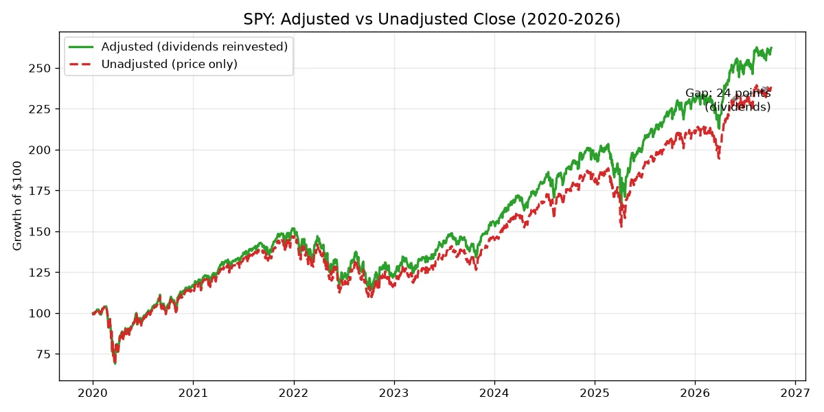
The backtest gap (+15.2%) is smaller than the buy-and-hold gap because the strategy isn’t always invested — it misses some dividends while in cash. But the direction is the same, and the lesson is blunt: a backtest on unadjusted data systematically understates any strategy that holds dividend-paying assets. You’re not being conservative; you’re being wrong.
And dividends are the friendly corporate action. Splits are worse — not because they’re subtle, but because they’re violent. When Apple did its 4:1 split in August 2020, the unadjusted price fell 75% overnight. A backtest on raw prices sees a -75% day and either triggers every stop-loss you’ve ever written or — if you’re “lucky” — generates a buy signal on a price that never existed.
2. Corporate Actions: Splits & Dividends
Three ways to handle corporate actions, and when each is right:
| Method | What it does | Use when |
|---|---|---|
| Backward-adjusted (default) | Past prices scaled down by all future splits/dividends; most recent price = actual market price | Backtesting. Your signals, returns, and recent prices all look real. This is what you want 95% of the time. |
| Forward-adjusted | Future prices scaled up; earliest price = actual | Almost never in backtesting. Useful for some tax accounting. |
| Unadjusted | Raw exchange prices, gaps and all | Only if you model corporate actions explicitly (e.g. you’re testing a dividend-capture strategy and need the actual cash flows). |
yfinance gives you backward-adjusted data with a single flag:
import yfinance as yf

# Adjusted (what you want for backtesting)
df = yf.download("SPY", auto_adjust=True, progress=False)

# Raw (only if you know why you need it)
df_raw = yf.download("SPY", auto_adjust=False, progress=False)
One honest caveat: adjustment is not free information. Backward-adjusted prices before a split are synthetic — they’re the price as if the split had always been in effect. For return calculations this is exactly right. But if your strategy uses price levels (e.g. “buy when price crosses $100”), adjusted history can generate signals at levels the stock never actually traded. Level-based strategies on long histories deserve a second look at what the adjusted prices imply.
Our data.py makes the safe choice the default:
from data import load_and_clean

# Adjusted, tz-aware, sanity-checked. One call.
df = load_and_clean("SPY", start="2020-01-01", end="2026-10-06")
adjust=True is the default. Passing adjust=False works, but you’re on your own — the docstring says so.
3. Missing Data & Alignment
Real data has holes. Exchanges close. Tickers get halted. Your vendor’s feed drops a bar. What you do with the hole matters more than you’d think.
The ffill trap
The tempting fix is forward-fill: carry the last price forward so there are no NaNs. On intraday data during a brief feed outage, that’s defensible. On daily bars, it’s dangerous:
- A halted stock flatlines for days. Your backtest sees a tradeable price every day. It wasn’t.
- A delisted stock’s last price repeats forever. Your “hold until the end” backtest happily values a dead company at its last print.
Our load_and_clean() defaults to fill="none" — leave the NaN, warn loudly, force you to decide. "ffill" exists but the warning tells you exactly why you’re playing with fire. "drop" is the middle ground.
# Default: NaNs stay, warning tells you how many
df = load_and_clean("SPY", fill="none")

# Explicit ffill — you asked for it, you own the consequences
df = load_and_clean("SPY", fill="ffill")
Multi-symbol alignment
The moment you hold two symbols, you need them on the same clock. SPY and QQQ both trade on NYSE, so this is easy — but the principle generalizes:
from data import align_symbols

frames = {
    "SPY": load_and_clean("SPY", start="2024-01-01", end="2024-06-30"),
    "QQQ": load_and_clean("QQQ", start="2024-01-01", end="2024-06-30"),
}
aligned = align_symbols(frames, how="inner")
# 124 common bars — every timestamp exists in BOTH symbols
Two design decisions worth knowing:
-
Timezone normalization happens at load. Every frame comes back tz-aware (UTC by default).
align_symbolsrefuses naive indexes — comparing a tz-naive New York close to a tz-naive London close is a bug that looks like a feature. -
how="inner"is the default. Only timestamps where every symbol traded survive. A half-day session that one symbol sat out gets excluded from all of them."outer"(union) exists for cases where you need the full calendar, but then you’re responsible for the NaNs.
4. Survivorship Bias
The nastiest data bug isn’t in your download code — it’s in your universe construction.
If you test a strategy on “the S&P 500” using today’s constituents, you’re testing on winners. The companies that went bankrupt, got acquired, or were demoted to small-cap purgatory aren’t in your sample. Your backtest never had the chance to lose money on them.
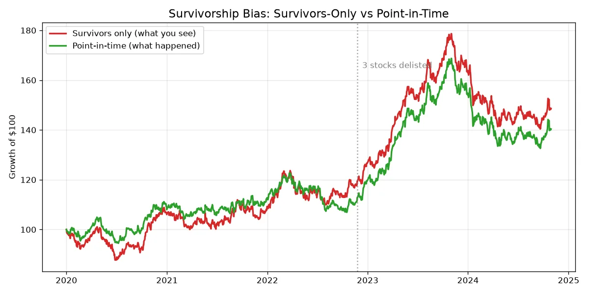
How big is the effect? A toy demo — ten stocks, five years, three delisted in year three:
| Universe | CAGR |
|---|---|
| Honest (point-in-time: hold what’s alive each day) | 7.0% |
| Survivors only (today’s winners, backfilled) | 8.2% |
| Bias | +1.2%/year |
1.2% per year, every year, from nothing but universe construction. On a real 20-year backtest of a stock-picking strategy, published estimates of survivorship bias run 1–3% annually — enough to turn a mediocre strategy into a publishable one.
The fix is point-in-time data: at each date, your universe must contain only what was knowable then. For index strategies, that means historical constituent lists (expensive). For single-ETF work like this series, the bias doesn’t apply — SPY can’t be delisted in the relevant sense. But the moment you graduate to stock selection, this is the first thing to get right, because it’s the bias that flatters you most while being hardest to see.
Run the demo yourself — data_demo.py prints all three demos (adjusted vs raw, survivorship, alignment) with real Yahoo data.
5. Merge Into the Toolkit: data.py
This tutorial isn’t a standalone trick — it’s Part 3 of a system we’re building together. The data logic now lives as the third module of goosos/quant-toolkit:
from quant_toolkit.data import load_and_clean, align_symbols
from quant_toolkit.backtest import run_backtest, ma_crossover_signals, summary

# Clean data in, honest backtest out
df = load_and_clean("SPY", start="2020-01-01")
price = df["Close"]
entries, exits = ma_crossover_signals(price, fast=20, slow=50)
pf = run_backtest(price, entries, exits)
print(summary(pf))
Why a toolkit, not just scripts? Each tutorial in this series adds one module. By Part 10 you’ll have backtest, validation, data, overfitting, metrics, costs, and sizing — a research system you understand line by line, because you watched every line get written. That’s the difference between using a library and owning your process.
Next: Part 4: PBO & Deflated Sharpe adds
overfitting.py— the statistics of not fooling yourself when you test hundreds of variants.
FAQ
Adjusted or unadjusted — which should I actually use?
Adjusted (backward-adjusted), unless you have a specific reason not to. The 15.2-point backtest gap in this tutorial is the cost of getting it wrong, and it always points the same direction: unadjusted understates.
My data vendor doesn’t offer adjusted prices. What now?
Get the corporate action history (splits and dividends with ex-dates) and adjust yourself: divide all prices before each event by the adjustment factor. It’s ~20 lines. Or switch vendors — any vendor without adjustment isn’t serious about backtesting.
How do I know if my data has gaps?
df["Close"].isna().sum() — and our load_and_clean() warns you by default. The dangerous gaps aren’t the ones you see; they’re the ones your pipeline silently filled.
Does survivorship bias affect ETF backtests?
Barely. An ETF is a fixed, tradable instrument — it can’t be “delisted” in the way a stock can (and if it liquidates, that’s a real, observable event in your data). The bias bites when your universe is selected ex-post: “top 100 stocks by market cap” as of today, backtested 10 years.
What about timezone alignment for crypto (24/7) vs equities?
Crypto trades every hour of every day; equities don’t. align_symbols(how="inner") on a BTC/SPY pair keeps only equity-market hours — which is usually what you want (no equity price exists at 3am Sunday). If you need the full crypto calendar, use how="outer" and handle equity NaNs explicitly.
References
- goosos/data-cleaning-tutorial — full code for this article.
- goosos/quant-toolkit — the growing toolkit;
data.pyis the Part 3 module. - yfinance documentation: corporate action handling via
auto_adjust. - Bailey, D. H., & López de Prado, M. (2014). The Deflated Sharpe Ratio. — Part 4’s foundation; selection bias compounds data bias.
Further Reading
- Part 1: VectorBT Tutorial — the backtest this series builds on; adds
backtest.py. - Part 2: Walk-Forward Analysis — in-sample vs out-of-sample; adds
validation.py. - Part 4: PBO & Deflated Sharpe (upcoming) — adds
overfitting.py.
Part 3 of Build Your Own Quant Research System · Code: goosos/data-cleaning-tutorial · Toolkit: goosos/quant-toolkit
