📦 Part 8 of Build Your Own Quant Research System — follow the series and you’ll build a complete, modular research toolkit from scratch, one tutorial at a time.
✅ Tested: vectorbt 1.1.1 · Python 3.12 · Last verified: 2026-10-08 · Update policy
📊 Market snapshot (as of 2026-10-08): SPY $777.22 · QQQ $757.73 · BTC $82,946 · ETH $2,571 — for context on when this was written.
In Part 1 through Part 7, we’ve built and stress-tested one strategy at a time. This tutorial changes the game: run several strategies together.
Here’s the pitch in one sentence: a portfolio of uncorrelated strategies has a higher Sharpe than any of its components. Not because the strategies got better — because their mistakes cancel out.
This is the only free lunch in finance. And like every free lunch, it comes with fine print.
Risk note: Everything here is educational. Diversification reduces volatility; it doesn’t eliminate risk, and it famously fails exactly when you need it most (more on that below). Nothing in this article is investment advice.
1. Why Portfolios Beat Single Strategies
Three strategies on SPY, same period, same honest costs. Watch what happens when we combine them:
| Strategy | Total return | Sharpe |
|---|---|---|
| MA(20,50) | +27.21% | +0.86 |
| MA(10,30) | +33.17% | +1.10 |
| RSI(14) | +36.10% | +1.01 |
| Portfolio (Sharpe-weighted) | — | +1.35 |
Best single strategy: Sharpe 1.10. The portfolio: 1.35. A +0.25 lift — from the same three strategies, no new alpha, just combination.
The math is simple. Portfolio variance isn’t the average of variances — it’s the average minus a diversification term driven by correlation:
σ²_portfolio = Σ wᵢ²σᵢ² + ΣΣ wᵢwⱼσᵢσⱼρᵢⱼ
When correlations (ρ) are low, the cross-terms shrink, and portfolio volatility drops faster than portfolio return. Lower volatility, same return → higher Sharpe. That’s the whole trick.
The key insight: you don’t need better strategies. You need different strategies. A mediocre strategy that’s uncorrelated with your book can add more value than a great strategy that’s correlated with it.
2. Correlation: The Only Thing That Matters
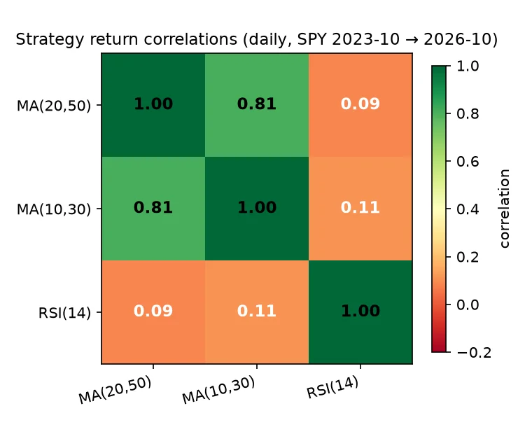
The heatmap tells the whole story:
- MA(20,50) vs MA(10,30): 0.81. Two trend-following moving-average strategies on the same asset. Of course they’re correlated — they’re the same idea with different parameters. Adding the second MA to the first is like adding a second umbrella to your bag: comforting, useless.
- RSI(14) vs either MA: ~0.10. Mean-reversion vs trend-following. When trend strategies bleed in choppy markets, RSI harvests the chop. When RSI gets run over by a trending market, the MAs ride it. This is diversification.
from portfolio import strategy_corr_matrix

corr = strategy_corr_matrix({
    "MA(20,50)": ma205_returns,
    "MA(10,30)": ma1030_returns,
    "RSI(14)": rsi_returns,
})
#           MA(20,50)  MA(10,30)  RSI(14)
# MA(20,50)      1.00       0.81     0.09
# MA(10,30)      0.81       1.00     0.11
# RSI(14)        0.09       0.11     1.00
The crisis trap: correlations are estimated on normal data. In a crash, correlations spike toward 1.0 — everything sells off together. Your beautifully diversified portfolio becomes one big correlated bet exactly when diversification matters most. This isn’t a flaw in the math; it’s a fact about markets. Size your portfolio for the crisis correlation, not the calm one.
How to read a correlation matrix in practice:
– Above 0.7: same trade, don’t count it as diversification.
– 0.3–0.7: partial diversification, useful but modest.
– Below 0.3: genuine diversifier — this is what you’re hunting for.
– Negative: rare and precious, but check why before trusting it.
3. Weighting Schemes
Once you have uncorrelated strategies, how much capital goes to each? Three standard answers:
from portfolio import equal_weight, sharpe_weight, inverse_vol_weight

w_eq  = equal_weight(3)
# → [0.33, 0.33, 0.33]

w_sh  = sharpe_weight([0.86, 1.10, 1.01])
# → [0.29, 0.37, 0.34] — more to higher Sharpe, zero to negative

w_iv  = inverse_vol_weight([0.0996, 0.0910, 0.1082])
# → [0.33, 0.36, 0.31] — more to calmer strategies
Equal weight (1/N): the robust default. No estimation, no overfitting. Decades of research show 1/N beats optimized weights out-of-sample — because optimized weights fit noise (Part 4).
Sharpe-weighted: allocate proportionally to (positive) Sharpe. Intuitive — back your winners. But Sharpe estimates are noisy, so you’re weighting by a noisy number. Our sharpe_weight() clips negatives to zero rather than shorting losers.
Inverse-volatility (“risk parity lite”): weight by 1/vol so each strategy contributes equal risk. Calmer strategies get more capital. Sensible when strategies have wildly different volatilities.
Now the honest result — all three schemes on our data:
| Scheme | Weights (MA20/MA10/RSI) | Portfolio Sharpe |
|---|---|---|
| Equal | 0.33 / 0.33 / 0.33 | +1.34 |
| Sharpe-weighted | 0.29 / 0.37 / 0.34 | +1.35 |
| Inverse-vol | 0.33 / 0.36 / 0.31 | +1.33 |
+1.33, +1.34, +1.35. The weighting scheme barely matters. This is itself the lesson: once you have low correlation, how you weight is second-order. The first-order decision was which strategies to combine. Don’t optimize the garnish when the meal is what counts.
4. Reality Check: Our Three-Strategy Portfolio
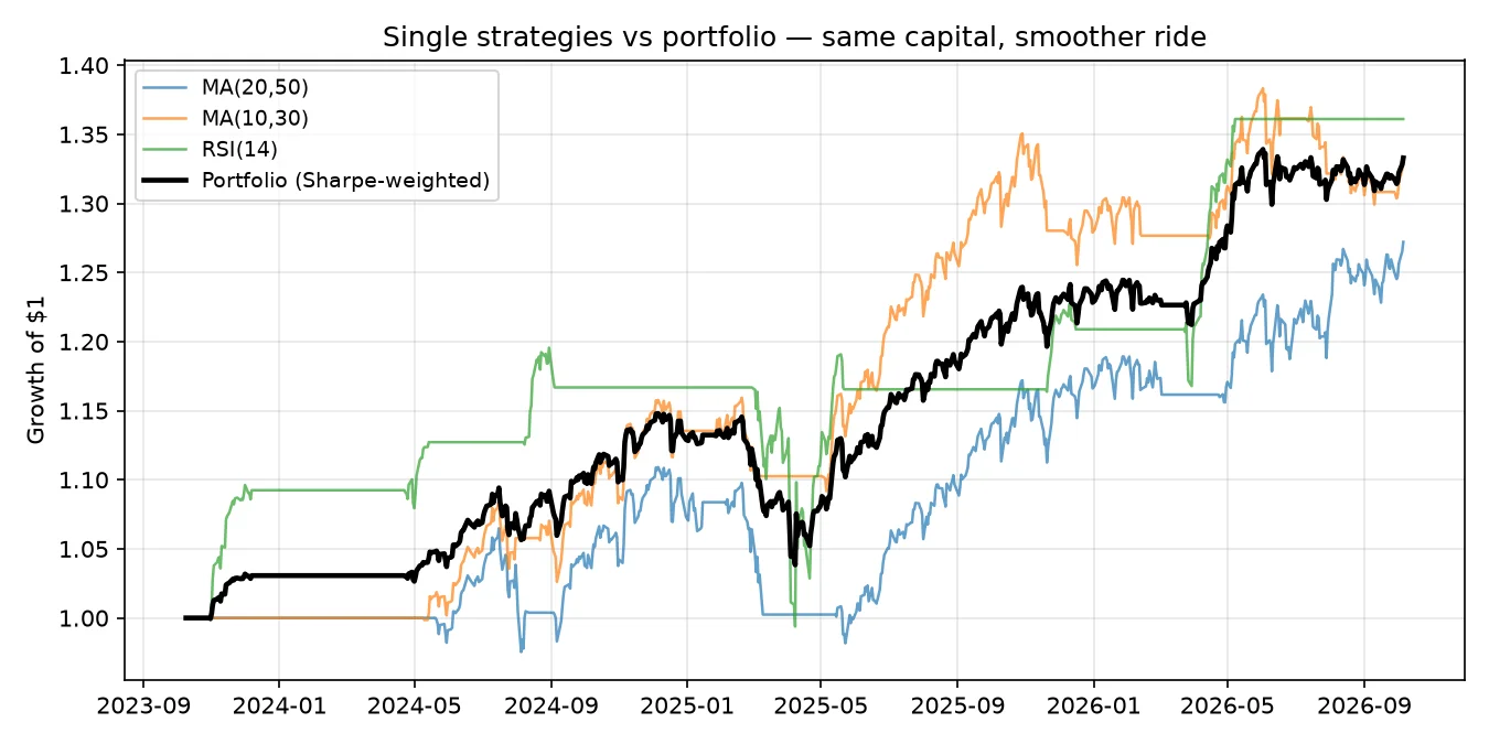
The chart shows it visually: the black portfolio line is smoother than any single strategy. Same capital, less drama, higher Sharpe.
Three honest takeaways:
1. The lift is real but modest: +1.10 → +1.35. Diversification added +0.25 Sharpe. That’s meaningful — over a decade, it compounds — but it didn’t turn a mediocre book into a great one. If your single strategies are bad, the portfolio is a diversified collection of bad.
2. The diversifier did the work, not the weighting. RSI’s ~0.10 correlation with the MAs is what lifted the portfolio. The two MAs (0.81 correlated) added almost nothing to each other. Lesson: one uncorrelated strategy beats three correlated ones. When evaluating a new strategy, the first question isn’t “what’s its Sharpe?” — it’s “what’s its correlation with my book?”
3. What this backtest doesn’t show. Daily rebalancing to target weights costs money (Part 6). Crisis correlations spike (Section 2). And with only 751 bars, our correlation estimates have wide error bars (Part 4 again). The +0.25 lift is a point estimate, not a promise.
The honest verdict: multi-strategy portfolios work, but the mechanism is specific — uncorrelated return streams. Two trend strategies on the same asset is one strategy wearing a disguise. Hunt for genuine behavioral difference (trend vs mean-reversion, different assets, different timeframes), verify the correlation is structural rather than lucky, and keep the weighting simple.
5. Merge Into the Toolkit: Composing What You Built
This tutorial adds no new module — and that’s the point. Everything here composes modules you already own:
from quant_toolkit.backtest import run_backtest, ma_crossover_signals
from quant_toolkit.metrics import sharpe
from quant_toolkit.costs import COST_TIERS
# portfolio.py is the recipe; the ingredients are Parts 1–7
portfolio.py is a recipe, not an ingredient. It shows how backtest (Part 1), metrics (Part 5), and costs (Part 6) snap together into something none of them is alone. That’s what a toolkit is for: the value isn’t in any single module, it’s in the composition.
Why a toolkit, not just scripts? Each tutorial in this series adds one module. By Part 10 you’ll have backtest, validation, overfitting, costs, sizing, data, and metrics — a research system you understand line by line, because you watched every line get written. That’s the difference between using a library and owning your process.
Next: Part 9: Parameter Robustness — when a parameter stops working, and how to know before it costs you.
FAQ
How many strategies do I need?
Fewer than you think, if they’re genuinely uncorrelated. Our three-strategy portfolio got most of its lift from one diversifier (RSI). Five correlated strategies add less than two uncorrelated ones. Quality of difference beats quantity of strategies.
Should I optimize the weights (mean-variance optimization)?
Probably not. Markowitz optimization is notoriously fragile — it maximizes sensitivity to estimation error. It treats your noisy Sharpe estimates as truth and concentrates on the noisiest winner. Equal weight or inverse-vol gets you 95% of the benefit with none of the overfitting. (Part 4 explains why.)
What about different assets, not just different strategies on SPY?
Even better — asset diversification is the classic use case. But the same rule applies: check the correlation matrix. SPY and QQQ are 0.9+ correlated; adding QQQ to SPY is barely diversification. SPY and TLT (bonds) or GLD (gold) is where the diversification lives.
Does diversification work in crypto?
Less well. In risk-off events, crypto correlations spike toward 1.0 — BTC, ETH, and alts all fall together. Diversification within crypto is weak; diversification between crypto and other asset classes is where it helps.
How often should I rebalance?
Rarely enough that costs don’t eat the benefit. Our demo assumes frictionless daily rebalancing — unrealistic (Part 6). Monthly or threshold-based rebalancing (only when weights drift >5%) captures most of the benefit at a fraction of the cost.
References
- Markowitz, H. (1952). Portfolio Selection. The Journal of Finance — the original mean-variance framework.
- DeMiguel, V., Garlappi, L., & Uppal, R. (2009). Optimal Versus Naive Diversification. Review of Financial Studies — 1/N beats optimization out-of-sample.
- goosos/portfolio-tutorial — full code for this article.
- goosos/quant-toolkit — the growing toolkit; this part composes existing modules.
Further Reading
- Part 1: VectorBT Tutorial — the backtest engine underneath.
- Part 2: Walk-Forward Analysis — in-sample vs out-of-sample.
- Part 3: Data Cleaning & Alignment — garbage in, garbage out.
- Part 4: Backtest Overfitting — PBO & Deflated Sharpe.
- Part 5: Performance Metrics — Sharpe vs Sortino vs Calmar.
- Part 6: Slippage & Commissions — the hidden tax.
- Part 7: Position Sizing — how much to bet.
- Part 9: Parameter Robustness — when parameters stop working.
Part 8 of Build Your Own Quant Research System · Code: goosos/portfolio-tutorial · Toolkit: goosos/quant-toolkit · Next: Part 9: Parameter Robustness
