📦 Part 2 of Build Your Own Quant Research System — follow the series and you’ll build a complete, modular research toolkit from scratch, one tutorial at a time.
✅ Tested: vectorbt 1.1.1 · Python 3.12 · yfinance 1.7.0 · Last verified: 2026-10-07 · Update policy
📊 Market snapshot (as of 2026-10-07): SPY $779.09 · QQQ $759.66 · BTC $83,700 · ETH $2,579 — for context on when this was written.
In Part 1, we backtested a moving-average crossover on SPY and got a Sharpe of 1.03. Five trades, 80% win rate, 27% total return. Looks great on paper.
Here’s the uncomfortable question Part 1 didn’t ask: how much of that Sharpe would you have actually captured if you’d traded it live?
The honest answer is almost always “less” — sometimes dramatically less. The gap between a backtest number and live-trading reality has a name: it’s the difference between in-sample and out-of-sample performance. And the standard tool for measuring it is walk-forward analysis.
This tutorial gives you the concept, the code, and — most importantly — the honest numbers for our Part 1 strategy. Spoiler: they hurt a little. That’s the point.
Risk note: Everything here is educational. Backtests are hypothetical — they don’t predict future returns, and a good backtest doesn’t mean a profitable strategy. Nothing in this article is investment advice.
1. The In-Sample Trap
Let’s be precise about what Part 1 actually measured.
We took three years of SPY data (October 2023 to October 2026), computed a 20/50 moving-average crossover, and ran one backtest over the entire period. Every number in the tearsheet — the 1.03 Sharpe, the 27% return, the -11.5% max drawdown — was computed on data the strategy “saw” during its construction.
Wait — did it? We didn’t optimize the (20, 50) parameters; we just picked the textbook defaults. So where’s the in-sample bias?
It’s subtler than parameter-picking. The bias is in the decision to publish. Think about it:
- We chose MA crossover because it’s a well-known strategy (survivorship bias of ideas — thousands of failed ideas never become tutorials).
- We chose SPY because it’s the most liquid ETF (we didn’t test 500 random tickers and report only the winner — but many people do exactly that).
- We chose a 3-year window that happens to include a strong bull market.
None of these are cheating. But they all mean the 1.03 Sharpe is conditional on choices made with knowledge of the outcome. A trader in October 2023 couldn’t have known that (20, 50) on SPY over the next three years would print 1.03.
This is the in-sample trap: any backtest result is optimistic to the degree that your research process touched the data. The only cure is testing on data that played no role — not in parameter selection, not in strategy selection, not in the decision to keep going.
That’s what “out-of-sample” means. And walk-forward analysis is the most practical way to get it.
2. Walk-Forward: How It Works
The idea is simple enough to explain in one paragraph:
Divide your history into alternating train and test windows. On each train window, you do whatever research you want — pick parameters, select indicators, make decisions. Then you run the resulting strategy on the test window only, and record the result. Roll the windows forward. Your out-of-sample performance is the collection of test-window results.
It’s called “walk-forward” because the windows walk forward through time, exactly the way live trading would: at each point, you only know the past.
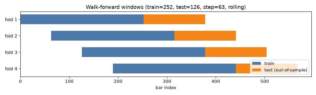
Two flavors:
| Rolling | Anchored | |
|---|---|---|
| Train window | Fixed size, slides forward | Starts at bar 0, grows each fold |
| Memory | Forgets old data (adapts to regime change) | Remembers everything (more data, slower to adapt) |
| Best for | Markets with regime shifts | Stable markets, more statistical power |
| This tutorial | ✅ Used | Mentioned for completeness |
Three parameters control everything:
- train_size — bars per training window. Too short and your parameter estimates are noise; too long and you’re slow to adapt. One year (252 trading days) is a sane default for daily data.
- test_size — bars per out-of-sample window. This is your “live trading” simulation per fold. A quarter (63 days) to half a year (126 days) is typical.
- step — how far windows advance each fold. Set it equal to
test_sizefor non-overlapping test segments (cleanest statistics).
One more honest detail: some folds will have zero trades. A slow strategy like MA(20,50) on a 63-day test window often doesn’t generate a single crossover. That’s not a bug — it’s information. A Sharpe ratio computed on zero trades is undefined, not zero, so we skip those folds and say so. (Our code does this explicitly.)
Three walk-forward mistakes beginners make
1. Test windows shorter than your strategy’s heartbeat. If your strategy trades ~5 times a year, a 1-month test window will be empty most folds. Rule: each test window should contain at least 3–5 trades on average, or your fold statistics are noise. When in doubt, lengthen the test window before adding more folds.
2. Overlapping test windows without accounting for it. If step < test_size, test segments overlap, and the fold results aren’t independent — your “10 folds” might carry the information of 4. Non-overlapping (step == test_size) keeps the statistics clean. Overlap is sometimes necessary with short histories; just don’t pretend overlapping folds are independent evidence.
3. Peeking at the full-period chart when choosing windows. “The strategy worked great 2023–2025 but died in 2026, so I’ll use 2024–2026 as my test range” — congratulations, you’ve just done in-sample selection on your out-of-sample design. Choose window sizes from principle (trade frequency, data length), not from staring at the equity curve. If you caught yourself doing this, re-read section 1.
3. Code: validation.py
Two functions. That’s the whole module.
walk_forward_splits() is a pure index generator — no prices, no strategies, just window arithmetic. It yields (train_idx, test_idx) integer indexers, so it works with any pandas-indexed data:
from validation import walk_forward_splits

# 751 bars, 1-year train, half-year test, rolling
for train_idx, test_idx in walk_forward_splits(751, 252, 126, step=63):
    print(f"train {train_idx[0]}-{train_idx[-1]}, "
          f"test {test_idx[0]}-{test_idx[-1]}")
train 0-251, test 252-377
train 63-314, test 315-440
train 126-377, test 378-503
...
run_walk_forward() does the actual work: it takes precomputed (and shifted — no lookahead, same rule as Part 1) entry/exit signals, slices them to each test window, backtests only that segment with Part 1’s run_backtest(), and returns a DataFrame with one row per fold:
from validation import run_walk_forward
from backtest import run_backtest, ma_crossover_signals  # Part 1 module

entries, exits = ma_crossover_signals(price, fast=20, slow=50)

wf = run_walk_forward(price, entries, exits,
                      train_size=252, test_size=126, step=63,
                      freq="1D")
print(wf[["test_start", "test_end", "sharpe", "n_trades"]])
The full module is ~120 lines, in validation.py. Design notes worth knowing:
- Signals are precomputed once on the full series (shifted one bar, per Part 1’s no-lookahead rule), then sliced per fold. This is correct because the shift already prevents lookahead — slicing a shifted signal can’t leak the future.
- Parameters are held fixed across folds. A stricter walk-forward would re-select parameters on each train window. We deliberately don’t, because this tutorial isolates one question: how much of the in-sample Sharpe survives unseen data? Parameter re-selection is selection-bias territory — that’s Part 4 (PBO & Deflated Sharpe).
- Empty folds are skipped with a comment, not silently zeroed. A skipped fold is honest; a fabricated zero Sharpe is a lie that flatters the average.
4. Reality Check: MA Strategy Out-of-Sample
Time for the honest numbers. Same data as Part 1 (SPY daily, October 2023 to October 2026, 751 bars), same MA(20,50) strategy, same honest costs (0.1% fees, 0.05% slippage per side).
In-sample (Part 1 method — one backtest, full period):
| Metric | Value |
|---|---|
| Total return | 27.21% |
| Sharpe | 1.03 |
| Max drawdown | -11.49% |
| Win rate | 80.0% (4 of 5 trades) |
| Profit factor | 4.35 |
Out-of-sample (walk-forward — 1-year train, half-year test, rolling, 4 folds with trades):
| Test window | Total return | Sharpe | Max DD | Trades |
|---|---|---|---|---|
| 2024-10-09 → 2025-04-10 | -7.50% | -2.46 | -8.68% | 1 |
| 2025-01-10 → 2025-07-14 | -1.98% | -0.43 | -10.57% | 2 |
| 2025-04-11 → 2025-10-10 | +11.06% | +2.72 | -2.98% | 1 |
| 2026-01-13 → 2026-07-15 | +5.84% | +1.62 | -4.49% | 1 |
Summary: mean out-of-sample Sharpe 0.36 — 35% of the in-sample 1.03. Half the folds lost money.
Let that sink in. The strategy didn’t “break” — two folds were solidly positive. But the in-sample number overstated reality by roughly 3×. And with only 1–2 trades per half-year window, every fold is a coin flip wearing a Sharpe ratio costume.
Three takeaways:
-
The gap is the finding. In-sample 1.03 → out-of-sample 0.36 is not a failure of the strategy; it’s a measurement of how much optimism was baked into the single-backtest number. Every strategy you test has this gap. Walk-forward is how you see it before your money does.
-
Slow strategies need long test windows. With 1–2 trades per fold, individual fold Sharpes are noise (-2.46 to +2.72 is a huge range). This is honest but low-resolution. A strategy that trades weekly would give you tighter fold estimates — one more reason to know your strategy’s trade frequency before trusting any single metric.
-
“Still positive on average” is not a buy signal. Mean OOS Sharpe 0.36 with 2 of 4 folds negative is not a strategy I’d trade. It’s a strategy I’d keep researching — maybe with a trend filter, maybe on a basket of assets instead of single-name SPY. The walk-forward didn’t kill the idea; it priced it correctly.
Run it yourself: walkforward_demo.py prints exactly these tables. Your numbers will differ slightly (Yahoo data updates daily), but the shape — in-sample flatters, out-of-sample disciplines — will be the same.
5. Merge Into the Toolkit: validation.py
This tutorial isn’t a standalone trick — it’s Part 2 of a system we’re building together. The walk-forward logic now lives as the second module of goosos/quant-toolkit:
from quant_toolkit.backtest import run_backtest, ma_crossover_signals, summary
from quant_toolkit.validation import walk_forward_splits, run_walk_forward

entries, exits = ma_crossover_signals(price, fast=20, slow=50)

# The Part 1 number (in-sample)
pf = run_backtest(price, entries, exits)
print("in-sample:", summary(pf)["sharpe"])

# The honest number (out-of-sample)
wf = run_walk_forward(price, entries, exits, train_size=252, test_size=126)
print("out-of-sample mean:", wf["sharpe"].mean())
What changed from the tutorial script? One thing: the toolkit version imports from quant_toolkit.backtest directly (no standalone fallback). The tutorial repo keeps a try/except import so python walkforward_demo.py works without installing anything — clone, pip install -r requirements.txt, run.
Why a toolkit, not just scripts? Each tutorial in this series adds one module. By Part 10 you’ll have backtest, validation, overfitting, costs, sizing, data, and metrics — a research system you understand line by line, because you watched every line get written. That’s the difference between using a library and owning your process.
Next: Part 3: Data Cleaning & Alignment, PBO & Deflated Sharpe adds
overfitting.py— the statistics of not fooling yourself when you test hundreds of variants.
FAQ
Walk-forward vs k-fold cross-validation — what’s the difference?
K-fold shuffles data randomly, which leaks the future into the past (a 2025 test fold trains on 2026 data). Walk-forward respects time order — train windows always precede their test windows. For time series, k-fold is wrong; walk-forward is the correct generalization.
How do I choose train/test/step sizes?
Rules of thumb for daily data: train ≥ 1 year (enough for parameter estimates to stabilize), test = 1 quarter to 1 year (long enough for your strategy to actually trade), step = test_size (non-overlapping tests = cleanest stats). Then sanity-check: if most folds have zero trades, your test window is too short for your strategy’s frequency.
Should I re-optimize parameters on each train window?
That’s the stricter version (“walk-forward optimization”), and it’s the right thing to do before trading. But it introduces selection bias — picking the best of N parameter sets on each window inflates results. Part 4 covers how to correct for that (PBO, Deflated Sharpe). This tutorial holds parameters fixed to isolate the pure in-sample/out-of-sample gap.
My out-of-sample Sharpe is negative. Is my strategy dead?
Not necessarily — check the trade count first. With 1–2 trades per fold, a negative Sharpe is noise, not signal. You need either more folds, longer test windows, or a faster strategy before concluding anything. What the negative does tell you: the in-sample number was not a promise.
Can I use walk-forward for machine learning models?
Yes — it’s the standard approach (often called “time-series split” in sklearn: TimeSeriesSplit). Same principle: never let future data touch training. The walk_forward_splits() function in this tutorial yields plain integer indexers, so it works with any model, not just vectorbt.
Why did you skip folds with no trades instead of counting them as zero?
Because Sharpe on zero trades is undefined, not zero. Inserting zeros would drag the mean toward zero and flatter the strategy (a losing strategy looks less bad). Skipping is honest; the article reports how many folds were skipped.
References
- Bailey, D. H., & López de Prado, M. (2014). The Deflated Sharpe Ratio: Correcting for Selection Bias in Backtests. — the statistical foundation for Part 4; explains why in-sample Sharpes overstate.
- López de Prado, M. Advances in Financial Machine Learning (2018), Chapter 7 (Cross-Validation in Finance) — purged k-fold CV and why standard cross-validation fails on financial time series.
- vectorbt documentation: vectorbt.pro — the backtesting engine used in Parts 1–2.
- goosos/walkforward-tutorial — full code for this article.
- goosos/quant-toolkit — the growing toolkit;
validation.pyis the Part 2 module.
Further Reading
- Part 1: VectorBT Tutorial — the backtest this article validates; adds
backtest.py. - Part 3: Data Cleaning & Alignment, PBO & Deflated Sharpe (upcoming) — adds
overfitting.py: correcting for selection bias when you test many variants.
Part 2 of Build Your Own Quant Research System · Code: goosos/walkforward-tutorial · Toolkit: goosos/quant-toolkit · Next: Part 3: Data Cleaning & Alignment
