VectorBT Tutorial: Backtest a Strategy in 30 Minutes

📦 Part 1 of Build Your Own Quant Research System — follow the series and you’ll build a complete, modular research toolkit from scratch, one tutorial at a time.

✅ Tested: vectorbt 1.1.1 · Python 3.12 · yfinance 0.2.40 · Last verified: 2026-10-07 · Update policy

📊 Market snapshot (as of 2026-10-07): SPY $779.09 · QQQ $759.66 · BTC $83,746 · ETH $2,580 — for context on when this was written.

If you’ve ever waited 20 minutes for a backtest to finish scanning 50 parameter combinations, you already know why VectorBT exists.

Most backtesting libraries — backtrader, zipline — are event-driven: they simulate the market bar by bar, like replaying history in real time. It’s realistic, but it’s slow. VectorBT takes the opposite approach: it’s vectorized. Your entire strategy becomes array operations over pandas Series, compiled by Numba, and 10,000 parameter combinations finish in seconds.

This tutorial takes you from zero to a complete, honest backtest in about 30 minutes:

Install VectorBT (v1.1.1, current as of October 2026)
Download free market data
Backtest a moving-average crossover strategy — full runnable code
Read the tearsheet: Sharpe, max drawdown, win rate — what the numbers actually mean
Scan thousands of parameters and plot a heatmap
Add realistic costs (the step most tutorials skip)
Dodge the three traps that silently inflate results

All code in this article is tested and runs end-to-end. The complete scripts live in the companion repo: goosos/vectorbt-tutorial.

Risk note: Everything here is educational. Backtests are hypothetical — they don’t predict future returns, and a good backtest doesn’t mean a profitable strategy. Nothing in this article is investment advice.

1. Why VectorBT (and When Not to Use It)

Three Python backtesting libraries dominate in 2026, and they solve different problems:

Library	Style	Best for	Status (2026)
VectorBT	Vectorized	Research speed: scan thousands of configs in seconds	Active, v1.1.1
backtrader	Event-driven	Realistic simulation for strategies headed to live trading	Maintained, v1.9.78
backtesting.py	Event-driven, simple API	Gentlest learning curve, single-strategy tests	Active, v0.6.6

VectorBT’s computation model is well-understood: independent implementations of the same strategies in event-driven engines produce matching fills at declared precision. The difference between the libraries is how they compute, not whether the math is trustworthy.

Use VectorBT when: you’re in the research phase — testing ideas, scanning parameters, comparing indicator settings. Speed is the whole point.

Don’t use VectorBT when: you need tick-level realism — order book dynamics, partial fills, latency modeling. That’s event-driven territory (backtrader), and eventually a paper-trading phase.

One more thing worth knowing upfront: VectorBT’s license changed. It’s no longer MIT — it’s Fair Code (Apache 2.0 + Commons Clause). Free for individuals and organizations to use, but you can’t sell a product that’s primarily VectorBT itself. For learning and research, nothing changes.

2. Installation

You need Python 3.11 or newer (3.10 was dropped in v1.1.0). Then:

pip install -U vectorbt

That’s the core. Two optional extras worth knowing:

pip install -U "vectorbt[full]"   # + TA-Lib, pandas-ta, and friends
pip install -U "vectorbt[rust]"   # Rust engine — skips Numba JIT warmup

Heads-up about the first run: VectorBT compiles its hot loops with Numba on first use. Your first backtest will pause for ~30–60 seconds while it compiles. Every run after that is fast. This is normal — don’t kill the process thinking it hung.

Verify the install:

import vectorbt as vbt
print(vbt.__version__)   # expect 1.1.1 or newer

3. Getting Free Data

VectorBT ships a Yahoo Finance wrapper, which is still the fastest path to real data:

import vectorbt as vbt

data = vbt.YFData.download("SPY")
price = data.get("Close")
print(price.head())
print(f"{len(price)} daily bars")

A few notes from experience:

Yahoo data is free but flaky — if a download fails, pip install -U yfinance usually fixes it, or just retry. (Our test script in the repo includes a synthetic-data fallback so the tutorial never hard-crashes on a bad network day.)
auto_adjust=True gives you split/dividend-adjusted closes — use it, or your long-run returns will be wrong.
Need crypto or multi-symbol? vbt.YFData.download(["BTC-USD", "ETH-USD"]) returns a DataFrame, and everything below broadcasts across columns automatically. There are also vbt.BinanceData, vbt.CCXTData, and vbt.AlpacaData connectors.

For this tutorial we’ll use 3 years of daily SPY — liquid, long history, no survivorship games.

4. Your First Backtest: MA Crossover

The strategy couldn’t be simpler: go long SPY when the 20-day moving average crosses above the 50-day, exit when it crosses back below. It’s a trend-following classic — not because it’s profitable (spoiler: the results are honest, not miraculous), but because it’s the perfect vehicle for learning the machinery.

Here’s the complete script. Copy it, run it, it works:

import vectorbt as vbt

# --- 1. Data ---
data = vbt.YFData.download("SPY", period="3y", interval="1d")
price = data.get("Close")

# --- 2. Signals ---
fast_ma = vbt.MA.run(price, 20)
slow_ma = vbt.MA.run(price, 50)

entries = fast_ma.ma_crossed_above(slow_ma)
exits = fast_ma.ma_crossed_below(slow_ma)

# Act on the NEXT bar — see Section 8 for why this line matters
entries = entries.vbt.signals.fshift(1)
exits = exits.vbt.signals.fshift(1)

# --- 3. Backtest ---
pf = vbt.Portfolio.from_signals(
    price, entries, exits,
    fees=0.001,      # 0.1% commission per side — realistic
    freq="1D",        # daily bars: annualizes Sharpe correctly
)

# --- 4. Results ---
print(pf.stats())

Run it. On our test machine (October 2026, SPY daily, Oct 2023 → Oct 2026, 752 bars) it printed:

Total return : 38.46%
Sharpe ratio : 1.29
Max drawdown : -11.31%
Win rate     : 83.33%  (6 trades)

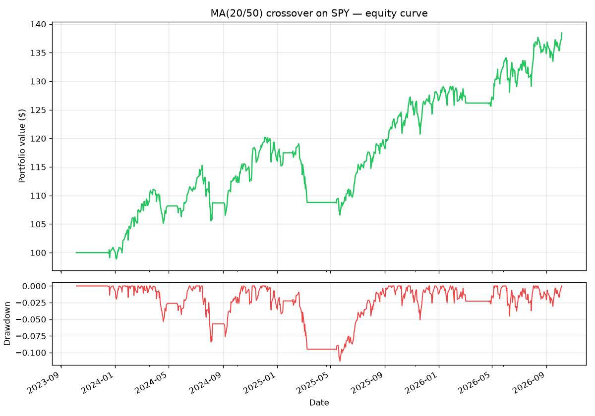
Six trades in three years, 38% total return, Sharpe 1.29. Respectable — and notably not the 500%-return fantasy that zero-fee tutorials produce. That’s the point: honest inputs, honest outputs.

The chart tells the rest of the story. Add this to plot the equity curve with drawdown:

import matplotlib
matplotlib.use("Agg")  # headless-safe
import matplotlib.pyplot as plt

fig, (ax1, ax2) = plt.subplots(2, 1, figsize=(10, 7),
                               sharex=True,
                               gridspec_kw={"height_ratios": [3, 1]})
pf.value().plot(ax=ax1, lw=1.5)
ax1.set_title("MA(20/50) crossover on SPY — equity curve")
ax1.set_ylabel("Portfolio value ($)")
ax1.grid(alpha=0.3)

pf.drawdown().plot(ax=ax2, color="#ef4444", lw=1.2)
ax2.set_ylabel("Drawdown")
ax2.grid(alpha=0.3)
fig.tight_layout()
fig.savefig("equity.png", dpi=120)

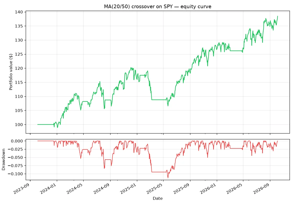
Figure: equity curve (top) and underwater drawdown (bottom) for the MA(20/50) crossover on SPY. Generated by the tutorial script — your numbers will differ slightly depending on the download date.

4b. Code Walkthrough: What Each Line Does

If you copied the script and it ran, great. Now let’s make sure you understand why each part exists — because the next time something breaks, this is the mental model that fixes it.

Data loading:

data = vbt.YFData.download("SPY", period="3y", interval="1d")
price = data.get("Close")

YFData.download is a thin wrapper around yfinance. The result is a Data object; .get("Close") pulls the adjusted close as a pandas Series indexed by date. Everything downstream — indicators, signals, portfolio — operates on this Series. If your data has gaps or NaNs, every indicator after it inherits the problem. When in doubt, price.isna().sum() first.

Indicators:

fast_ma = vbt.MA.run(price, 20)
slow_ma = vbt.MA.run(price, 50)

vbt.MA.run computes a moving average and returns an Indicator object. The .ma attribute holds the actual Series, but you rarely touch it directly — the object exposes signal methods like .ma_crossed_above(). Think of it as “indicator + its natural operations” bundled together.

Signals:

entries = fast_ma.ma_crossed_above(slow_ma)
exits = fast_ma.ma_crossed_below(slow_ma)

These return boolean Series: True on bars where the crossover happened. Note what they don’t contain: no prices, no position sizes, no “how much to buy.” VectorBT separates signal generation (your strategy logic) from portfolio simulation (how signals become trades). This separation is what makes parameter scanning trivial later — you swap the signals, the portfolio engine stays the same.

The shift:

entries = entries.vbt.signals.fshift(1)
exits = exits.vbt.signals.fshift(1)

Covered in depth in Section 8, but the one-line version: without this, you’re trading on information from the future. .vbt.signals.fshift(1) is VectorBT’s signal-aware shift — it moves signals forward one bar so today’s signal trades tomorrow.

The portfolio:

pf = vbt.Portfolio.from_signals(
    price, entries, exits,
    fees=0.001,
    freq="1D",
)

from_signals is the workhorse. It takes your price and signal Series and simulates the entire portfolio: cash, positions, fees, equity curve. The returned pf object is your laboratory — every metric, plot, and trade record in the rest of this tutorial comes from it.

Try it yourself: change fees=0.001 to fees=0.0 and re-run. Watch the Sharpe change. That delta is the cost of realism.

5. Reading the Tearsheet: What the Numbers Actually Mean

pf.stats() dumps ~25 metrics. Most beginners stare at Total Return and stop. Here’s how to read the four that matter, using our real numbers:

Total Return: 38.46%
Over three years, that’s roughly 11.5% annualized. Sounds fine — until you ask what SPY itself did. Always compare against buy-and-hold: pf.benchmark_return() gives you that baseline. A strategy that underperforms buy-and-hold with more complexity isn’t a strategy, it’s a hobby.

Sharpe Ratio: 1.29
Return per unit of volatility, annualized. Rough guide: below 1.0 is noise, 1.0–2.0 is decent, above 2.0 in a real backtest deserves skepticism (or a closer look at the assumptions). Our 1.29 says “this did something right, but it’s not magic.” Note: Sharpe is only correct because we passed freq="1D" — without it, VectorBT can’t annualize and the number is silently wrong. More on this in Section 8.

Max Drawdown: −11.31%
The worst peak-to-trough loss. This is the number that determines whether you can actually hold the strategy. A −11% drawdown is uncomfortable; a −40% drawdown ends most retail accounts psychologically long before it ends mathematically. Drawdown, not return, is what kills strategies in practice.

Win Rate: 83.33% (5 of 6 trades)
High win rate, few trades. Don’t be seduced: with 6 trades, one loser swings this number by 17 points. Win rate without trade count is marketing. Also check Profit Factor (pf.trades.profit_factor()) — gross profit divided by gross loss. Above 1.5 is healthy; below 1.2 is fragile.

Three metrics beginners misread most:

Total Return without the benchmark — always ask “vs. what?”
Sharpe without checking freq — wrong annualization is silent
Win rate without trade count — 83% of 6 trades means almost nothing; 55% of 600 trades means a lot

Useful accessors for your own exploration:

pf.total_return()        # 0.3846
pf.sharpe_ratio()        # 1.29
pf.max_drawdown()        # -0.1131
pf.trades.win_rate()     # 0.8333
pf.trades.profit_factor()
pf.trades.expectancy()
pf.trades.records_readable  # every trade as a DataFrame

Beyond the big four: pf.stats() also reports Calmar Ratio (annualized return ÷ max drawdown — how much return you got per unit of pain), Omega Ratio (probability-weighted gains vs. losses — captures asymmetry Sharpe misses), and Sortino Ratio (like Sharpe but only penalizes downside volatility). For a first backtest you don’t need all three, but know they exist: when Sharpe and Sortino disagree sharply, your returns have a fat downside tail worth investigating.

Expectancy deserves a special mention: pf.trades.expectancy() tells you the average profit per trade in dollars. Multiply it by your expected trade frequency and you get a rough sense of whether the strategy is worth the operational hassle. A strategy with $2 expectancy that trades twice a year is a curiosity; the same expectancy at 200 trades a year is a business.

5b. Troubleshooting: Errors You’ll Actually Hit

TypingError: non-precise type array(pyobject, 1d, C)
You built signals with raw pandas and a .shift(1). The NaN at position 0 converted your boolean Series to object dtype, and Numba can’t compile that. Fix: .fillna(False).astype(bool) — or better, use vbt.MA.run() and .vbt.signals.fshift(1) as this tutorial does.

First run hangs for ~60 seconds
That’s Numba JIT compilation, not a hang. Go make tea. It only happens once per fresh Python process.

yfinance download returns empty
Yahoo changes their API every year or two and yfinance breaks for a few days. Run pip install -U yfinance first. If you’re behind a corporate proxy, the download may fail silently — our repo script falls back to synthetic data with a clear warning so the tutorial never dead-ends.

Sharpe looks absurdly high (>5)
You probably forgot freq. Without it, VectorBT annualizes on the wrong timescale. Check that freq matches your bar size: "1D" for daily, "1h" for hourly.

Heatmap shows all NaN
Your slow window exceeds your data length, or missing_index="drop" misaligned multi-symbol data. Print price.shape and your window range first.

6. Parameter Scanning: VectorBT’s Killer Feature

Here’s where VectorBT earns its keep. Instead of testing one (20, 50) pair, test every fast/slow combination from 2 to 100 — 9,801 backtests — in a single pass:

import numpy as np

windows = np.arange(2, 101)
fast_ma, slow_ma = vbt.MA.run_combs(price, window=windows, r=2,
                                    short_names=["fast", "slow"])
entries = fast_ma.ma_crossed_above(slow_ma).vbt.signals.fshift(1)
exits = fast_ma.ma_crossed_below(slow_ma).vbt.signals.fshift(1)

pf = vbt.Portfolio.from_signals(price, entries, exits,
                                fees=0.001, freq="1D")

sharpe = pf.sharpe_ratio()
print("Best:", sharpe.idxmax(), "->", sharpe.max())

Then visualize it as a heatmap:

fig = pf.total_return().vbt.heatmap(
    x_level="fast_window", y_level="slow_window",
    trace_kwargs=dict(colorbar=dict(title="Total return")))
fig.show()   # or fig.write_image("heatmap.png")

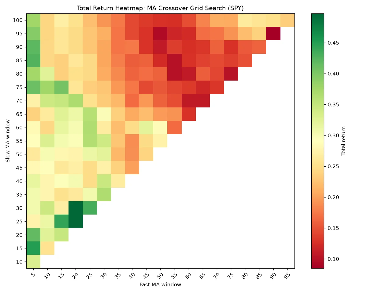
Figure: total return across fast/slow MA combinations on SPY. Look for a broad plateau of good parameters (robust) vs. a single sharp peak (overfit). Generated by parameter_scan.py.

Now read the heatmap like a researcher, not a tourist:

A broad plateau of good parameters (e.g., fast 15–30, slow 40–70 all work) → the edge is probably real. Small changes don’t break it.
A single sharp peak surrounded by mediocrity → you’ve found noise, not signal. That exact (17, 63) combo won’t survive contact with new data.

This is the visual intuition behind overfitting, and it’s the reason our content plan has a dedicated article on it: Backtest Overfitting, PBO & Deflated Sharpe (coming next). VectorBT even ships a built-in deflated Sharpe ratio — pf.returns().vbt.returns.deflated_sharpe_ratio(...) — which penalizes Sharpe for the number of trials you ran. Use it after any grid search.

Try it yourself: change the scan to np.arange(5, 201, 5) and see how the plateau shifts. Then add slippage=0.0005 and watch the best Sharpe drop — that’s reality entering the chat.

7. Costs: The Step Most Tutorials Skip

VectorBT’s defaults are fees=0.0 and slippage=0.0. A zero-cost backtest is a fantasy backtest — and it’s the default, so most copy-paste tutorials silently publish fantasies.

Our script already sets fees=0.001 (10 basis points per side — roughly realistic for retail). Watch what happens when you compare:

pf_free = vbt.Portfolio.from_signals(price, entries, exits, freq="1D")
pf_real = vbt.Portfolio.from_signals(price, entries, exits,
                                     fees=0.001, slippage=0.0005, freq="1D")

print(f"Fantasy Sharpe: {pf_free.sharpe_ratio():.2f}")
print(f"Realistic Sharpe: {pf_real.sharpe_ratio():.2f}")
print(f"Fees paid: ${pf_real.stats()['Total Fees Paid']:.2f}")

For a low-turnover strategy like ours (6 trades), costs barely dent the result. For a strategy that trades daily, 10bps per side compounds into a massacre. Rule of thumb: if adding realistic costs flips your Sharpe from green to red, you never had a strategy — you had a commission-donation plan.

You can also set sensible defaults once, globally:

vbt.settings['portfolio']['fees'] = 0.0005
vbt.settings['portfolio']['slippage'] = 0.0002

7b. Position Sizing: The Multiplier Nobody Talks About

So far our backtest uses VectorBT’s default: size=np.inf, meaning “use all available cash.” That’s fine for learning, but position sizing is where real strategies live or die — a great signal with reckless sizing still blows up.

VectorBT gives you precise control:

# Fixed fractional: risk 10% of equity per trade
pf = vbt.Portfolio.from_signals(
    price, entries, exits,
    size=0.10, size_type="percent",
    fees=0.001, freq="1D",
)

# Fixed dollar amount per trade
pf = vbt.Portfolio.from_signals(
    price, entries, exits,
    size=1000, size_type="value",   # $1000 per trade
    fees=0.001, freq="1D",
)

The size_type options:

`size_type`	Meaning	When to use it
`"amount"` (default)	Number of shares/contracts	You think in share counts
`"value"`	Dollar value per trade	Fixed-dollar risk
`"percent"`	Fraction of current equity	Compounding strategies
`"targetpercent"`	Rebalance to target %	Portfolio allocation

Why this matters for the tutorial strategy: our MA crossover with size=np.inf goes all-in on every signal. Try size=0.5, size_type="percent" — half the capital per trade, the rest in cash. The Sharpe often improves because drawdowns shrink faster than returns. That’s a free lesson in risk management from one parameter change.

Try it yourself: run the backtest with size=1.0, 0.5, and 0.25 (percent). Plot all three equity curves on one chart. Notice how the shape changes — that’s position sizing doing more work than your entry signal.

A word on leverage: VectorBT supports it (leverage parameter), but this tutorial won’t demonstrate it. Leverage multiplies both returns and the speed at which mistakes kill you. Master unleveraged backtesting first.

8. Three Traps That Silently Inflate Results

Trap 1: Lookahead bias (the `fshift(1)` line)

VectorBT fills a signal on the same bar, at that bar’s close, by default. But your signal was computed from that bar’s close — information you wouldn’t have had until the bar ended. Trading on it is time travel.

The fix: shift signals forward one bar (decide at today’s close, trade tomorrow), or fill at the open:

entries = entries.vbt.signals.fshift(1)   # our choice
# — or —
pf = vbt.Portfolio.from_signals(price, entries, exits, price=open_price)

Bonus gotcha we hit while testing: if you write the shift with raw pandas — (fast_ma > slow_ma).shift(1) — the NaN at position 0 silently converts the boolean Series to object dtype, and VectorBT’s Numba engine explodes with a cryptic TypingError. The fix is .fillna(False).astype(bool). Using vbt.MA.run() + .vbt.signals.fshift(1) avoids this entirely — another reason to use the library’s own signal methods.

Trap 2: Forgetting `freq`

Without freq="1D", Sharpe, annualized return, and Calmar are computed on the wrong timescale — silently. No error, no warning, just wrong numbers. Set it every time. (For hourly bars: freq="1h".)

Trap 3: The zero-fee default

Covered in Section 7, but it bears repeating because it’s the most common sin in VectorBT tutorials online: from_signals(price, entries, exits) with no fees, no slippage, no freq. Three missing arguments, three layers of fantasy.

8b. Putting It Together: A 10-Minute Research Workflow

Here’s the workflow this tutorial has been building toward. Next time you have a strategy idea, run this loop:

Step 1: One clean backtest (5 min)
Write the simplest version. One asset, one parameter set, realistic fees, fshift(1), freq set. If the Sharpe is below 0.5 at this stage, the idea probably isn’t worth optimizing — move on.

Step 2: Parameter scan (2 min)
Grid-scan the key parameters. Look at the heatmap. Ask: is there a plateau, or just a peak? Plateau → proceed. Lone peak → discard; you found noise.

Step 3: Cost sensitivity (1 min)
Double the fees and slippage. If the strategy survives, it’s robust to your cost estimates being wrong (they will be). If it dies, your edge was thinner than your uncertainty.

Step 4: Position sizing (2 min)
Try size=0.5, size_type="percent". Compare Sharpe and max drawdown against all-in. Most beginners are surprised how often half-size wins on risk-adjusted terms.

Total: 10 minutes from idea to a defensible answer. That’s the VectorBT superpower — not the library itself, but the iteration speed it gives your research process. The strategies that survive this loop earn the right to a walk-forward test (our next tutorial). The ones that don’t get discarded in minutes instead of weeks.

Try it yourself: pick a different indicator — RSI, Bollinger Bands, or Donchian channels (all in vbt.IF / vbt.BBANDS / vbt.DONCHIAN). Run the 4-step loop. Time yourself. That’s your new research cadence.

8c. Merge Into the Toolkit: `backtest.py`

This tutorial isn’t a standalone trick — it’s Part 1 of a system we’re building together. The core logic from this article now lives as the first module of goosos/quant-toolkit:

from quant_toolkit.backtest import run_backtest, ma_crossover_signals, summary

entries, exits = ma_crossover_signals(price, fast=20, slow=50)
pf = run_backtest(price, entries, exits)
print(summary(pf))
# {'total_return': 0.3846, 'sharpe': 1.29, 'max_drawdown': -0.1131, ...}

What changed from the tutorial script? Almost nothing — that’s the point:

run_backtest() wraps vbt.Portfolio.from_signals with honest defaults (fees, slippage, freq always set)
ma_crossover_signals() bundles signal generation + the one-bar shift (no lookahead, ever)
summary() returns the metrics that matter as a plain dict

Why a toolkit, not just scripts? Each tutorial in this series adds one module. By Part 10 you’ll have backtest, validation, overfitting, costs, sizing, data, and metrics — a research system you understand line by line, because you watched every line get written. That’s the difference between using a library and owning your process.

Next: Part 2: Walk-Forward Analysis adds validation.py — testing on data your parameter scan never saw.

9. Where to Go Next

You now have a complete, honest backtesting workflow — and the first module of your toolkit. Natural next steps:

Part 2: Walk-Forward Analysis (next in series) — adds validation.py: the antidote to overfitting.
Portfolio backtests — from_signals broadcasts across columns, so multi-asset portfolios are nearly free. Try SPY + TLT + GLD.
Stops — sl_stop=0.05, tp_stop=0.10 adds stop-loss/take-profit in one line. Measure whether they help or just add churn.
Part 4: Backtest Overfitting, PBO & Deflated Sharpe — adds overfitting.py: the methodology behind not fooling yourself.

The full code for this tutorial is in goosos/vectorbt-tutorial. The growing toolkit is in goosos/quant-toolkit. Clone them, break them, make them yours.

FAQ

Is VectorBT free?
Yes for learning and research. The open-source library is free under Fair Code licensing (not MIT anymore — commercial redistribution has restrictions). There’s a paid VectorBT Pro with new features, but everything in this tutorial uses the free version.

Can I use VectorBT for live trading?
Not directly — it’s a research/backtesting library, not a broker connector. The workflow is: research in VectorBT → validate realism in an event-driven engine or paper trading → execute through a broker API.

VectorBT vs backtrader — which should I learn?
Learn VectorBT first if your bottleneck is ideas (you need to test many). Learn backtrader if your bottleneck is realism (your strategy is headed to live trading). They’re complements, not rivals.

Why is the first run so slow?
Numba JIT compilation (~30–60s once). Subsequent runs are seconds. The [rust] extra avoids even that.

Does vbt.YFData.download still work?
Yes. Yahoo changes their API periodically and yfinance breaks for a few days; pip install -U yfinance is the usual fix.

How do I backtest a portfolio of multiple assets?
Pass a DataFrame instead of a Series: vbt.YFData.download(["SPY", "TLT", "GLD"]) gives you multi-column price data, and from_signals broadcasts everything automatically. Each column becomes an independent backtest — then use pf.resample() or groupby to aggregate.

Can VectorBT handle intraday/hourly data?
Yes — set freq="1h" (or "15m", etc.) and make sure your signals align to the same index. The vectorized engine doesn’t care about bar size; only the annualization math needs the right freq.

What’s the difference between from_signals and from_orders?
from_signals takes boolean entry/exit arrays (what this tutorial uses). from_orders takes explicit order sizes — more control, more work. Start with signals; graduate to orders when you need partial position management.

Why do my results differ from the article’s numbers?
Three reasons: (1) Yahoo data updates — your 3-year window covers different dates; (2) auto_adjust settings; (3) VectorBT version. Small differences are normal. Large differences mean something’s wrong — check freq first.

References

Polakow, O. — vectorbt GitHub repository. Source for API patterns, Portfolio.from_signals parameters, and v1.1.1 release notes cited in this tutorial.
VectorBT official documentation — indicator methods (MA.run, run_combs, ma_crossed_above), signal handling (.vbt.signals.fshift), and portfolio settings.
vectorbt on PyPI — version history (1.1.1, Sep 2026), Python requirement (≥3.11), and the Fair Code license notice.
Bailey, D. H. & López de Prado, M. (2014). “The Deflated Sharpe Ratio: Correcting for Selection Bias, Backtest Overfitting and Non-Normality.” Journal of Portfolio Management, 40(5), 94–107. SSRN. The statistical basis for the deflated Sharpe ratio discussed in Section 6.
López de Prado, M. (2018). Advances in Financial Machine Learning. Wiley. Chapter on backtest overfitting and the PBO framework referenced in our overfitting article.

VectorBT Tutorial: Backtest a Strategy in 30 Minutes

1. Why VectorBT (and When Not to Use It)

2. Installation

3. Getting Free Data

4. Your First Backtest: MA Crossover

4b. Code Walkthrough: What Each Line Does

5. Reading the Tearsheet: What the Numbers Actually Mean

5b. Troubleshooting: Errors You’ll Actually Hit

6. Parameter Scanning: VectorBT’s Killer Feature

7. Costs: The Step Most Tutorials Skip

7b. Position Sizing: The Multiplier Nobody Talks About

8. Three Traps That Silently Inflate Results

Trap 1: Lookahead bias (the `fshift(1)` line)

Trap 2: Forgetting `freq`

Trap 3: The zero-fee default

8b. Putting It Together: A 10-Minute Research Workflow

8c. Merge Into the Toolkit: `backtest.py`

9. Where to Go Next

FAQ

References

Further Reading

Leave a Comment Cancel reply

1. Why VectorBT (and When Not to Use It)

2. Installation

3. Getting Free Data

4. Your First Backtest: MA Crossover

4b. Code Walkthrough: What Each Line Does

5. Reading the Tearsheet: What the Numbers Actually Mean

5b. Troubleshooting: Errors You’ll Actually Hit

6. Parameter Scanning: VectorBT’s Killer Feature

7. Costs: The Step Most Tutorials Skip

7b. Position Sizing: The Multiplier Nobody Talks About

8. Three Traps That Silently Inflate Results

Trap 1: Lookahead bias (the fshift(1) line)

Trap 2: Forgetting freq

Trap 3: The zero-fee default

8b. Putting It Together: A 10-Minute Research Workflow

8c. Merge Into the Toolkit: backtest.py

9. Where to Go Next

FAQ

References

Further Reading

Leave a Comment Cancel reply

$ whoami

$ ls ./series

$ cat links.txt

Trap 1: Lookahead bias (the `fshift(1)` line)

Trap 2: Forgetting `freq`

8c. Merge Into the Toolkit: `backtest.py`