📦 Part 6 of Build Your Own Quant Research System — follow the series and you’ll build a complete, modular research toolkit from scratch, one tutorial at a time.
✅ Tested: vectorbt 1.1.1 · Python 3.12 · Last verified: 2026-10-08 · Update policy
📊 Market snapshot (as of 2026-10-08): SPY $777.22 · QQQ $757.73 · BTC $83,135 · ETH $2,579 — for context on when this was written.
In Part 1 we ran our MA crossover with “honest” costs: 0.1% commission and 0.05% slippage per side. In Part 2 through Part 5, those defaults quietly rode along in every backtest.
This tutorial asks: what exactly are those numbers, and what happens when they’re wrong?
Costs are the hidden tax on every strategy. They’re the reason a backtest showing Sharpe 1.5 can lose money live. They’re also the most boring part of quant research — which is exactly why most tutorials skip them, and why most beginners get blindsided.
Risk note: Everything here is educational. Cost models are approximations — real fills depend on your broker, order type, and market conditions. Nothing in this article is investment advice.
1. Why Costs Kill Strategies
Let’s start with our MA(20,50) strategy on SPY, run at three cost tiers:
| Tier | Per-side cost | Total return | Sharpe | Max DD |
|---|---|---|---|---|
| zero (fantasy) | 0 bps | 29.83% | 1.11 | -12.73% |
| honest | 15 bps | 28.09% | 1.06 | -13.25% |
| harsh | 30 bps | 26.37% | 1.00 | -13.77% |
Five trades over three years. Costs barely dent it — Sharpe drops from 1.11 to 1.00. Boring, right?
Now the twist: frequency changes everything. Our MA strategy trades ~1.7 times per year. Each round trip costs 30 bps at the “honest” tier. Total drag: ~0.5% per year. Negligible.
But imagine a strategy that trades weekly — 50 round trips a year. Same 30 bps per round trip. Total drag: 15% per year. A strategy with 12% gross edge becomes a -3% loser. Dead.
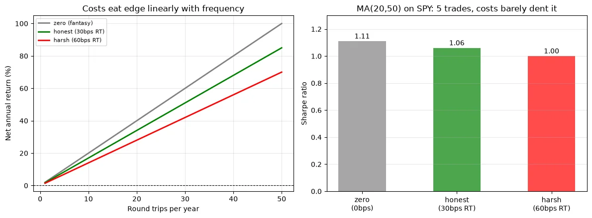
The math is brutal and simple:
Annual cost drag = round trips per year × cost per round trip
A 2%-edge strategy survives 6.7 round trips/year at honest costs, but only 3.3 at harsh costs. Double the cost, halve the viable frequency. This is why high-frequency strategies need institutional-grade execution — and why slow strategies like ours can afford to be sloppy.
The asymmetry nobody tells beginners: costs are the one component of a backtest you can estimate before trading. Returns are uncertain; costs are nearly certain. If your backtest is only profitable at zero costs, it’s not a strategy — it’s a fantasy.
2. Commissions: The Visible Part
Commissions are the easy part. Your broker tells you the rate. Two structures dominate:
Proportional (most common for stocks/ETFs): you pay a percentage of notional value per side. Interactive Brokers Pro charges ~0.05% with a $1 minimum (2026). So a $10,000 trade costs $5.
from costs import commission_pct

# $10k trade at 5 bps with $1 minimum (IBKR-like)
commission_pct(10_000, rate=0.0005, min_per_trade=1.0)
# → 5.0
Fixed (common for futures/options): flat fee per contract regardless of size. One ES futures contract might cost $2.50 round trip.
from costs import commission_fixed

commission_fixed(n_trades=4, per_trade=2.50)
# → 10.0
The gotcha with fixed commissions: they punish small accounts. A $2.50 fee on a $500 trade is 50 bps. On a $50,000 trade it’s 0.5 bps. This is why backtests should always use your account size, not a fantasy $1M.
Our TradeCost class bundles everything:
from costs import TradeCost

ibkr_like = TradeCost(commission_rate=0.0005, slippage_bps=5.0, min_commission=1.0)
print(f"Round trip: {ibkr_like.round_trip_pct()*100:.2f}%")
# → Round trip: 0.20%

# Plug straight into backtest
from backtest import run_backtest
pf = run_backtest(price, entries, exits, **ibkr_like.to_backtest_kwargs())
3. Slippage: The Invisible Killer
Slippage is the difference between the price you wanted and the price you got. It’s invisible because no statement line says “slippage: $47” — it just silently worsens every fill.
Three sources:
-
Bid-ask spread. You see SPY at $777.22 — that’s the mid. You buy at $777.25 (ask), sell at $777.19 (bid). On liquid ETFs the spread is 1–2 bps. On small caps it can be 50+ bps.
-
Market impact. Your order moves the price. Buying 10 shares of SPY: zero impact. Buying 100,000 shares: you are the market for a moment.
-
Timing lag. Your signal fires at the close. Your order fills seconds later at a slightly different price. In fast markets this dwarfs the spread.
Modeling approaches (simplest to most realistic):
from costs import slippage_fixed, slippage_vol

# Fixed: 5 bps adverse on every fill
slippage_fixed(777.22, bps=5.0)
# → 0.389 ($ per share)

# Volatility-proportional: scales with market stress
# cost = k × rolling_std(returns) × price
slippage_vol(price_series, returns_series, k=0.5, window=20)
The volatility model captures an important truth: slippage is worse when you most want to trade. Volatility spikes during the exact moments strategies generate signals (breakouts, crashes). Fixed slippage underestimates costs precisely when it matters.
Rule of thumb for daily strategies on liquid ETFs: 5–10 bps per side total (commission + slippage). For less liquid names: 20–50 bps. If you don’t know, use the harsh tier — it’s better to kill a marginal strategy in backtest than in production.
4. Reality Check: MA Strategy Net of Costs
Full picture for our MA(20,50) on SPY (751 bars, 5 trades):
| Metric | zero | honest (15bps/side) | harsh (30bps/side) |
|---|---|---|---|
| Total return | 29.83% | 28.09% | 26.37% |
| Sharpe | 1.11 | 1.06 | 1.00 |
| Max drawdown | -12.73% | -13.25% | -13.77% |
| Cost drag/year | 0.00% | ~0.58% | ~1.15% |
Three honest observations:
-
Slow strategies are cost-robust. Five trades in three years means costs are rounding error. This is a genuine advantage of low-frequency approaches — and one more reason beginners should start slow.
-
The ranking doesn’t change. Honest costs don’t flip our strategy from “good” to “bad.” But that’s because it’s slow. Run the same analysis on a strategy with 50 trades/year and the harsh tier would be fatal.
-
“Honest” is a choice. We picked 15 bps/side as our default in Part 1. That was a judgment call, not a measurement. Real IBKR fills on SPY might be 8 bps; a retail broker with payment for order flow might be effectively 15–20 bps. The right move: bracket your results — show zero, honest, and harsh, like we just did. If the strategy survives harsh, it’s robust. If it only works at zero, it’s decoration.
5. Merge Into the Toolkit: costs.py
This tutorial isn’t a standalone trick — it’s Part 6 of a system we’re building together. The cost logic now lives as the sixth module of goosos/quant-toolkit:
from quant_toolkit.backtest import run_backtest, ma_crossover_signals
from quant_toolkit.costs import TradeCost, COST_TIERS

entries, exits = ma_crossover_signals(price, fast=20, slow=50)

for name, tier in COST_TIERS.items():
    pf = run_backtest(price, entries, exits, **tier.to_backtest_kwargs())
    print(f"{name}: Sharpe {pf.sharpe_ratio():.2f}")
Why a toolkit, not just scripts? Each tutorial in this series adds one module. By Part 10 you’ll have backtest, validation, overfitting, costs, sizing, data, and metrics — a research system you understand line by line, because you watched every line get written. That’s the difference between using a library and owning your process.
Next: Part 7: Position Sizing adds
sizing.py— Kelly, volatility targeting, and why sizing matters more than signals.
FAQ
Should I use fixed or proportional commissions?
Match your broker. US stock/ETF brokers (IBKR, Schwab) are proportional with minimums. Futures/options are fixed per contract. When in doubt, model both and take the worse — costs are the one thing you want to overestimate.
How do I estimate slippage without live trading data?
Start with 5–10 bps per side for liquid ETFs, 20–50 bps for small caps. Better: use TAQ data or your broker’s execution reports once you paper trade. Best: assume harsh tier in research — if the strategy survives, it’s robust.
Does vectorbt model partial fills?
No — vectorbt assumes full fills at the (slippage-adjusted) signal price. For strategies where partial fills matter (large size relative to volume), you need an event-driven engine. That’s beyond our research scope.
Why not just add 1% costs and call it “conservative”?
Because arbitrary conservatism hides information. Showing three tiers (zero/honest/harsh) tells you how sensitive the strategy is to costs. A strategy that dies at honest costs but lives at zero is fragile; one that survives harsh is robust. One number can’t tell you that.
Do costs affect walk-forward results?
Yes — apply the same cost tier to every fold. Costs don’t change the walk-forward methodology, but they can flip individual fold results from positive to negative, which is honest and important.
References
- Interactive Brokers commission schedule (2026) — US stock/ETF pricing reference.
- Harris, L. Trading and Exchanges (2003), Chapter 3 — market microstructure: bid-ask spread, market impact.
- goosos/costs-tutorial — full code for this article.
- goosos/quant-toolkit — the growing toolkit;
costs.pyis the Part 6 module.
Further Reading
- Part 1: VectorBT Tutorial — the backtest this article cost-adjusts.
- Part 2: Walk-Forward Analysis — in-sample vs out-of-sample.
- Part 3: Data Cleaning & Alignment — garbage in, garbage out.
- Part 4: Backtest Overfitting — PBO & Deflated Sharpe.
- Part 5: Performance Metrics — Sharpe vs Sortino vs Calmar.
- Part 7: Position Sizing (upcoming) — adds
sizing.py.
Part 6 of Build Your Own Quant Research System · Code: goosos/costs-tutorial · Toolkit: goosos/quant-toolkit · Next: Part 7: Position Sizing
