📦 Part 9 of Build Your Own Quant Research System — follow the series and you’ll build a complete, modular research toolkit from scratch, one tutorial at a time.
✅ Tested: vectorbt 1.1.1 · Python 3.12 · Last verified: 2026-10-08 · Update policy
📊 Market snapshot (as of 2026-10-08): SPY $777.22 · QQQ $757.73 · BTC $82,790 · ETH $2,566 — for context on when this was written.
In Part 1 through Part 8, we’ve picked parameters, validated them, cost-adjusted them, and combined them. This tutorial asks an uncomfortable question about every parameter we’ve ever chosen: is it robust, or did we just get lucky?
Here’s the core idea in one sentence: a parameter that works at 20 but breaks at 21 is not a finding — it’s noise. Real edges are broad. If your strategy only works at exactly one parameter combination, the market will find a way to move you off it.
This is the last line of defense before Part 10 assembles the full system.
Risk note: Everything here is educational. Robustness testing reduces overfitting risk; it doesn’t eliminate it. A plateau in backtest can still be a mirage if the market regime changes. Nothing in this article is investment advice.
1. The Fragility Problem
Imagine two parameter choices for the same strategy:
- Choice A: Sharpe 1.62 at (fast=31, slow=33). Move to (32,33): Sharpe 0.9. Move to (31,34): Sharpe 0.7. A sharp spike.
- Choice B: Sharpe 0.92 at (fast=20, slow=50). Move ±2 in either direction: Sharpe stays between 0.83 and 0.95. A broad plateau.
Which would you trade with real money?
If you said B, you already understand parameter robustness. Choice A looks better on paper — 1.62 vs 0.92 — but it’s a peak: a single point where noise happened to align. Choice B is a plateau: a region where the strategy works across many nearby settings.
The intuition: markets are noisy, and your parameter estimates are noisy. If the truth is “somewhere around (20,50)” but you deploy exactly (31,33) because it backtested best, you’ve optimized for the noise, not the signal. The peak is the overfitting (Part 4) wearing a different mask.
The cliff vs plateau mental model: picture the Sharpe surface as terrain. A plateau means you can stumble a few steps in any direction and still stand on solid ground. A cliff means one wrong step and you fall off. Real trading will push you a few steps — regime shifts, estimation error, changing volatility. You want to start on flat ground.
2. Sensitivity Analysis
How do you measure fragility? Slice the parameter grid along one axis and watch how fast Sharpe degrades as you move away from the optimum.
from robustness import parameter_sensitivity, degradation_score

# Sharpe profile: vary fast window, slow fixed at 50
profile = parameter_sensitivity(grid, axis=0)  # grid is the (fast, slow) Sharpe matrix
print(profile.head())
# fast
# 10    0.41
# 11    0.52
# 12    0.58
# ...

score = degradation_score(profile)
# → 0.045: Sharpe drops ~4.5% per unit step away from the optimum
The degradation_score is the mean Sharpe loss per parameter step, normalized by the best Sharpe. Interpretation:
- Below 0.02: flat — the parameter barely matters. Robust.
- 0.02–0.05: gentle slope — normal. Most honest parameters live here.
- Above 0.05: cliff — small tweaks cause large damage. Fragile.
Our real grid: fast-axis degradation 0.045, slow-axis 0.027. The fast window is the touchier parameter — which makes sense, because the fast MA controls when you enter, and entry timing is where noise lives. The slow MA controls the trend filter, which is inherently smoother.
Why this matters more than the Sharpe itself: a Sharpe of 1.62 with degradation 0.15 is worse than a Sharpe of 0.92 with degradation 0.02. The first number is a photograph of luck; the second is a property of the strategy. Sensitivity analysis turns “what’s the best Sharpe?” into “how stable is the Sharpe?” — and stability is what survives contact with live markets.
3. The Plateau Test
Sensitivity profiles are one-dimensional. The plateau test looks at the full 2-D neighborhood: what fraction of nearby parameter combinations are within 90% of the reference Sharpe?
from robustness import find_plateau, plateau_neighbors

# Global view: how much of the whole grid is near the best?
mask, plateau_frac, is_peak = find_plateau(grid, frac=0.9)
# → plateau_frac = 0.003 (0.3%!), is_peak = True
# The grid's "best" is a lone spike. Red flag.

# Local view: is (20, 50) on flat ground?
frac, verdict = plateau_neighbors(grid, (20, 50), frac=0.9,
                                  radius=2, reference="local")
# → 1.00, "plateau": every neighbor within 90% of MA(20,50)'s own Sharpe

frac, verdict = plateau_neighbors(grid, (31, 33), frac=0.9,
                                  radius=2, reference="local")
# → 0.12, "peak": the "best" params are a fragile spike
Two reference modes, two different questions:
reference="global": is this parameter near the global optimum’s plateau? Useful for asking “am I leaving money on the table?”reference="local": is this parameter on flat ground? Useful for asking “will small changes break me?” This is the robustness question.
The rule of thumb: deploy parameters with a local verdict of "plateau" (≥80% of neighbors within 90%). Accept "slope" (40–80%) with caution — it works, but monitor it. Never deploy a "peak" (<40%) with real money, no matter how good the headline Sharpe looks.
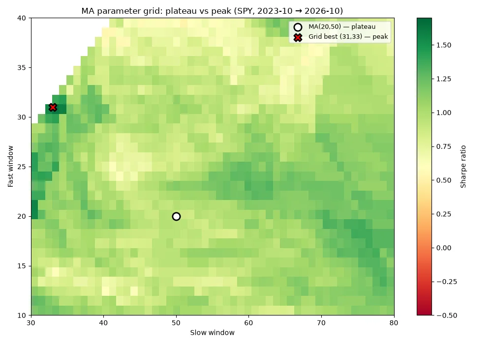
The heatmap makes it visual: MA(20,50) sits in a broad green region. The grid best (31,33) — marked with a red X — is an isolated bright pixel. One of these is a strategy. The other is a lottery ticket.
4. Reality Check: Is MA(20,50) on a Plateau or a Peak?
Full results from our 1,515-combination grid (SPY daily, 2023-10 → 2026-10, honest costs):
| Parameter | Sharpe | Global verdict | Local verdict |
|---|---|---|---|
| Grid best (31, 33) | 1.62 | PEAK (12%) | PEAK (12%) |
| MA(20, 50) | 0.92 | PEAK (0%) | PLATEAU (100%) |
Read it carefully, because it’s subtle:
- MA(20,50) is not the best. Its Sharpe (0.92) is far below the grid best (1.62). The “global PEAK” verdict just means it’s nowhere near the optimum’s neighborhood — which is fine, because the optimum’s neighborhood is a mirage.
- MA(20,50) is robust. 100% of its neighbors are within 90% of its own Sharpe. Nudge fast to 18 or 22, nudge slow to 48 or 52 — performance barely moves. That’s what you want.
- The grid best is fragile. (31,33) hits 1.62, but only 12% of its neighbors stay within 90%. Worse: fast=31 and slow=33 are suspiciously close together — nearly equal windows means the two MAs cross constantly on noise. That 1.62 is almost certainly whipsaw luck, not edge.
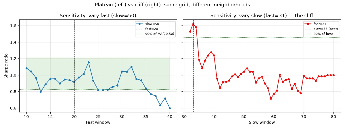
The profiles tell the same story in 1-D. Left: varying fast around 20 (slow=50) — flat, boring, reliable. Right: varying slow around 33 (fast=31) — a cliff. One step off the peak and Sharpe collapses.
The honest verdict: MA(20,50) was never the “optimal” parameter — and that’s exactly why it’s the right one to trade. We chose it in Part 1 for its economic intuition (a monthly vs quarterly trend filter), and the plateau test confirms the choice: it’s on solid ground. The optimizer’s pick (31,33) is a sharper number on a shakier foundation. In parameter selection, boring beats brilliant.
Three honest caveats: only 752 bars, so the grid itself is estimated with noise (Part 4 again). The plateau could shift in a different regime. And robustness is necessary but not sufficient — a robustly bad parameter is still bad.
5. Merge Into the Toolkit: Composing What You Built
This tutorial adds no new module — and that’s the point. Everything here composes modules you already own:
from quant_toolkit.backtest import run_backtest, ma_crossover_signals
from quant_toolkit.metrics import sharpe
from quant_toolkit.overfitting import deflated_sharpe
# robustness.py is the recipe; the ingredients are Parts 1-7
robustness.py is a recipe, not an ingredient. It shows how backtest (Part 1), metrics (Part 5), and overfitting (Part 4) snap together into a robustness screen none of them is alone. The plateau test is the practical sibling of Part 4’s PBO: PBO asks “did I overfit by selecting?”, the plateau test asks “did I overfit by locating?”
Why a toolkit, not just scripts? Each tutorial in this series adds one module. By Part 10 you’ll have backtest, validation, overfitting, costs, sizing, data, and metrics — a research system you understand line by line, because you watched every line get written. That’s the difference between using a library and owning your process.
Next: Part 10: Assembling the Full System — wiring all seven modules into one research pipeline, end to end.
FAQ
Isn’t the plateau test just eyeballing a heatmap?
The heatmap is the intuition; find_plateau() and plateau_neighbors() are the quantification. Eyeballing doesn’t scale to 4-D parameter spaces and doesn’t give you a number to put in a report. The verdicts (“plateau”/”slope”/”peak”) turn a visual habit into a testable rule.
What if my whole grid is a peak — no plateau anywhere?
Then you don’t have a strategy, you have a fitted curve. Go back to the drawing board: simpler signals, longer data, or accept that the edge isn’t there. A peak everywhere is the market telling you “no.”
Should I pick the center of the plateau?
Usually yes — maximum distance from the edges gives maximum tolerance for regime drift. But don’t overthink it: anywhere on the plateau is defensible. The point is to avoid peaks, not to micro-optimize within flat ground (that would be overfitting the robustness test itself).
How does this relate to walk-forward analysis (Part 2)?
Walk-forward tests temporal robustness (does it work out-of-sample?). The plateau test checks parameter robustness (does it work nearby?). A strategy needs both: walk-forward says “it worked later,” plateau says “it works around here.” Either one failing is a veto.
Can a parameter be on a plateau in backtest but fragile live?
Yes — if the regime changes. Plateaus are estimated on historical data; a volatility regime shift can reshape the terrain. That’s why Part 10 combines everything: plateau-tested parameters, walk-forward validated, honestly costed, sanely sized.
References
- Bailey, D. H., & López de Prado, M. (2014). The Deflated Sharpe Ratio. — the multiple-testing correction behind Part 4’s DSR; plateau testing is its geometric cousin.
- DeMiguel, V., Garlappi, L., & Uppal, R. (2009). Optimal Versus Naive Diversification. — cited in Part 8; the same “don’t over-optimize” moral applies to parameters.
- goosos/robustness-tutorial — full code for this article.
- goosos/quant-toolkit — the growing toolkit; this part composes existing modules.
Further Reading
- Part 1: VectorBT Tutorial — the backtest engine and original parameter grid.
- Part 2: Walk-Forward Analysis — temporal robustness.
- Part 3: Data Cleaning & Alignment — garbage in, garbage out.
- Part 4: Backtest Overfitting — PBO & Deflated Sharpe.
- Part 5: Performance Metrics — Sharpe vs Sortino vs Calmar.
- Part 6: Slippage & Commissions — the hidden tax.
- Part 7: Position Sizing — how much to bet.
- Part 8: Multi-Strategy Portfolios — combining strategies.
- Part 10: Assembling the Full System — the complete pipeline.
Part 9 of Build Your Own Quant Research System · Code: goosos/robustness-tutorial · Toolkit: goosos/quant-toolkit · Next: Part 10: Assembling the Full System
