📦 Part 7 of Build Your Own Quant Research System — follow the series and you’ll build a complete, modular research toolkit from scratch, one tutorial at a time.
✅ Tested: vectorbt 1.1.1 · Python 3.12 · Last verified: 2026-10-08 · Update policy
📊 Market snapshot (as of 2026-10-08): SPY $777.22 · QQQ $757.73 · BTC $82,886 · ETH $2,569 — for context on when this was written.
In Part 1 through Part 6, we’ve obsessed over what to trade: signals, validation, costs, metrics. This tutorial is about how much.
Position sizing is the least glamorous part of quant research. No fancy math, no machine learning, no alpha. And yet it’s the difference between a strategy that compounds for a decade and one that blows up in a bad quarter.
Here’s the uncomfortable truth: most backtests assume you’re fully invested, all the time. Real traders aren’t. The gap between “the strategy returned 27%” and “I made 27%” is entirely about sizing.
Risk note: Everything here is educational. Sizing math doesn’t eliminate risk — it manages it. Kelly in particular can suggest dangerously large bets; always use a fraction. Nothing in this article is investment advice.
1. Why Sizing Beats Signals
Same strategy, same signals, three different bet sizes. Watch what happens:
| Method | Total return | Sharpe | Max drawdown |
|---|---|---|---|
| Fixed 100% (fully invested) | 27.21% | 1.03 | -11.49% |
| Fixed 50% (half exposure) | 13.61% | 1.03 | -5.74% |
| Vol-target 15% | 2.58% | 0.94 | -0.31% |
This is our MA(20,50) on SPY, real data, honest costs. Three observations:
1. Halving size halves everything except Sharpe. 27% → 13.6% return, -11.5% → -5.7% drawdown, but Sharpe stays 1.03. Sizing is a scaling operation: it doesn’t create edge, it scales the edge you have (and the pain that comes with it).
2. The Sharpe invariance is the point. If someone shows you a Sharpe of 2.0, ask about the sizing. A Sharpe of 2.0 at 10% volatility is a very different beast than Sharpe 2.0 at 40% volatility. Sizing determines which one you experience.
3. Vol targeting tames drawdowns — at a cost. Our vol-targeted run cut max drawdown to nearly zero (-0.31%), but also crushed returns to 2.58%. When you’re only invested 30% of the time (5 trades in 3 years), vol targeting spends most of its time under-invested. It’s the right tool for always-on strategies, less so for slow ones.
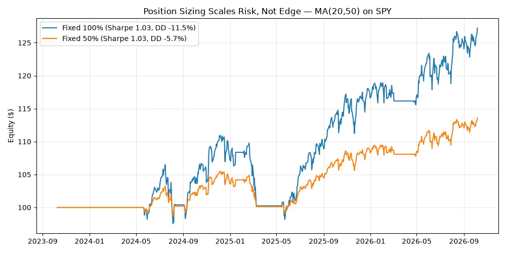
The chart tells the story visually: same shape, different amplitude. That’s all sizing does — and that’s everything.
The Kelly danger: Full Kelly maximizes long-run growth in theory. In practice, it produces drawdowns that most humans can’t stomach. Simulations show full-Kelly bettors face >50% drawdowns with disturbing regularity. The math is right; the psychology isn’t. Which is why professionals use half-Kelly or less.
2. Fixed Fractional & Kelly
Fixed fractional: the default
Bet X% of your equity on every trade. 100% = fully invested. 50% = half. That’s it.
from sizing import fixed_fractional

size = fixed_fractional(equity=100_000, fraction=0.5)
# → $50,000 position
Boring? Yes. But boring is robust: no parameters to overfit, no regime assumptions, no blowups from misestimated volatility. Most professional systematic funds use some variant of fixed fractional as their baseline.
Kelly: the optimal bet (that nobody should use at full size)
The Kelly criterion answers: what fraction maximizes long-run log wealth?
f* = p - (1 - p) / b
Where p = win probability, b = win/loss payoff ratio.
from sizing import kelly_fraction, half_kelly

# Our MA strategy: 80% win rate, avg win $8.83, avg loss $8.13
f = kelly_fraction(win_prob=0.80, win_loss_ratio=8.83/8.13)
# → 0.616 (full Kelly says bet 61.6%!)

safe = half_kelly(win_prob=0.80, win_loss_ratio=8.83/8.13)
# → 0.308 (half-Kelly: 30.8% — still aggressive)
Why half? Full Kelly assumes you know p and b exactly. You don’t — they’re estimated from 5 trades. Estimation error + full Kelly = overbetting = ruin. Half-Kelly cuts growth by ~25% but cuts volatility roughly in half. It’s the standard practitioner’s compromise.
When Kelly says zero (or negative): don’t bet. A negative Kelly fraction means no edge. This is a feature, not a bug — it’s the math telling you to sit out.
The honest caveat
Kelly was derived for repeated independent bets with known probabilities — coin flips, not markets. Markets have fat tails, regime changes, and estimation error. Treat Kelly as a sizing intuition (bet more when edge is large, less when uncertain), not a precise prescription.
3. Volatility Targeting
The idea: keep portfolio volatility constant. When markets get choppy, shrink positions. When calm, grow them.
from sizing import vol_target_size

size = vol_target_size(
    equity=100_000,
    returns=strategy_returns,  # pd.Series of daily returns
    target_vol=0.15,           # 15% annualized target
    lookback=63,               # 63-day trailing window
)
# Returns dollar size, clipped to [0, 100%]
How it works: each day, compute trailing realized volatility (63-day standard deviation, annualized). Size = target_vol / realized_vol. If realized vol doubles, size halves.
When it shines: always-on strategies (daily rebalancing, multi-asset portfolios). It prevents the classic problem where a quiet period lulls you into oversized positions right before volatility explodes.
When it struggles: slow, infrequent strategies like our MA crossover. With 5 trades in 3 years, the strategy is in cash most of the time. Vol targeting sees low realized vol (lots of zero-return days) and wants to increase size — exactly wrong for a strategy that’s mostly sitting out.
The lookback tradeoff: shorter lookback (21 days) reacts faster but whipsaws. Longer (126 days) is smoother but slow to adapt. 63 days (one quarter) is the common default.
4. Reality Check: MA Strategy Under Three Sizings
Let’s be precise about what sizing did and didn’t change:
| Fixed 100% | Fixed 50% | Vol-target 15% | |
|---|---|---|---|
| Total return | 27.21% | 13.61% | 2.58% |
| Sharpe | 1.03 | 1.03 | 0.94 |
| Max drawdown | -11.49% | -5.74% | -0.31% |
| Calmar | 0.79 | 0.79 | 2.77 |
Three takeaways:
1. Sizing is a risk dial, not an alpha dial. Sharpe barely moved (1.03 → 0.94). If your strategy has no edge, no sizing method creates one. If it does, sizing determines how much of that edge you capture — and how much pain you endure.
2. Drawdown scales linearly with size. Halve the size, halve the drawdown. This is the most actionable fact in this tutorial: if you can’t stomach -11.5%, don’t abandon the strategy — halve the size.
3. Vol targeting’s Calmar looks great (2.77) but don’t be fooled. The tiny drawdown (-0.31%) inflates the ratio. With only 2.58% total return, this isn’t a better strategy — it’s a strategy that’s barely invested. Calmar rewards low drawdowns even when they come from not trading.
The honest verdict: for our slow MA strategy, fixed fractional (somewhere between 50–100%) is the right call. Vol targeting is solving a problem we don’t have (we’re not overexposed to volatility spikes — we’re mostly in cash). Kelly says 30.8% half-Kelly, which is a reasonable sanity check but not something to follow mechanically with 5 data points.
5. Merge Into the Toolkit: sizing.py
This tutorial isn’t a standalone trick — it’s Part 7 of a system we’re building together. The sizing logic now lives as the seventh module of goosos/quant-toolkit:
from quant_toolkit.sizing import (
    fixed_fractional, kelly_fraction, half_kelly, vol_target_size,
)

# How much to bet?
size = fixed_fractional(equity=100_000, fraction=0.5)

# Is there edge?
f = half_kelly(win_prob=0.8, win_loss_ratio=1.09)
Why a toolkit, not just scripts? Each tutorial in this series adds one module. By Part 10 you’ll have backtest, validation, overfitting, costs, sizing, data, and metrics — a research system you understand line by line, because you watched every line get written. That’s the difference between using a library and owning your process.
Next: Part 8: Multi-Strategy Portfolios — combining strategies, correlation, and portfolio-level backtesting.
FAQ
Fixed fractional vs Kelly — which should I use?
Start with fixed fractional. It’s robust, transparent, and has no estimation risk. Add Kelly as a sanity check (if Kelly says 5%, your 100% fixed bet is probably too big). Graduate to vol targeting when you run multi-asset or always-on strategies.
Why half-Kelly and not quarter-Kelly?
Half is the conventional compromise. Quarter-Kelly is even safer but gives up more growth. The right fraction depends on your confidence in the edge estimates — with 5 trades of history, even half-Kelly is aggressive. There’s no formula for humility.
Does position sizing affect Sharpe?
No — scaling positions scales both returns and volatility proportionally, leaving Sharpe unchanged (as our demo showed: 1.03 at both 100% and 50%). Sizing changes how much Sharpe you experience, not the Sharpe itself. The exception: vol targeting can slightly change Sharpe because the scaling isn’t constant.
Can sizing turn a losing strategy profitable?
No. Sizing scales edge; it doesn’t create it. A negative-expectation strategy sized optimally still loses money — just more slowly. Fix the strategy first, size second.
What about pyramiding / adding to winners?
That’s a sizing tactic (position management), distinct from the strategic sizing in this tutorial. Pyramiding can improve returns but concentrates risk. It’s an advanced topic — get the basics right first.
References
- Kelly, J. L. (1956). A New Interpretation of Information Rate. Bell System Technical Journal — the original Kelly paper.
- Thorp, E. O. (2006). The Kelly Criterion in Blackjack, Sports Betting, and the Stock Market. — practical guide, covers half-Kelly rationale.
- goosos/sizing-tutorial — full code for this article.
- goosos/quant-toolkit — the growing toolkit;
sizing.pyis the Part 7 module.
Further Reading
- Part 1: VectorBT Tutorial — the backtest this article sizes.
- Part 2: Walk-Forward Analysis — in-sample vs out-of-sample.
- Part 3: Data Cleaning & Alignment — garbage in, garbage out.
- Part 4: Backtest Overfitting — PBO & Deflated Sharpe.
- Part 5: Performance Metrics — Sharpe vs Sortino vs Calmar.
- Part 6: Slippage & Commissions — the hidden tax.
- Part 8: Multi-Strategy Portfolios — combining strategies.
Part 7 of Build Your Own Quant Research System · Code: goosos/sizing-tutorial · Toolkit: goosos/quant-toolkit · Next: Part 8: Multi-Strategy Portfolios
